16. AGX Cable

The agxCable module is used to simulate cables, hoses, ropes, short wires and dress packs. These are long structures with a circular cross section that can be bent, stretched and twisted. The agxCable namespace provides the Cable class which uses a lumped elements approach to model such structures. By using agxCable::Cable it is possible to create simulations with cable structures that behave realistically in contacts and interaction with other simulated objects. This can be used, for example, for training operations of assembling scenarios, measurement of load and wear on cables in a robot scenario or for cable motion analysis in articulated devices.

16.1. Model

The lumped elements approach means that the cable is represented by a sequence of rigid bodies linked together using constraints. Each rigid body constitutes what is called a segment. Together the segments define the shape, extent and location of the cable. In addition to a rigid body, each segment has a geometry that allows it to collide with other geometries in the simulation, including other segments of the same cable. Each geometry contains a capsule and consecutive segments are placed with a bit of overlap so that the flat sides of facing hemispheres coincide in a straight cable.

Fig. 16.1 Two consecutive cable segments. Notice the overlap.

This makes the cable surface smoother at bends, compared to if cylinders had been used. The geometries for consecutive segments are exempted from contact generation. The cable is a one-dimensional structure and thus each constraint connects exactly two segments.

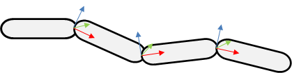
Fig. 16.2 A Cable consisting of four segments and three LockJoints (constraints).

Parameters and properties set on the cable are translated into parameters on these bodies and constraints. This makes it possible to create cables that range from easily bendable to completely stiff.

Both the bodies and the constraints operate on all six degrees of freedom, which makes it possible to track bending, twisting and stretching of the cable independently.

16.2. Cable vs Wire

agxWire is another very efficient AGX component that is used to simulate long, bendable structures. Whereas the cable has a fixed resolution, meaning that the number and size of the segments remain constant throughout the simulation, the wire has dynamic resolution. This is the main difference compared to agxWire, which can adjust the resolution locally in order to improve stability. This makes it possible to use agxWire in scenarios with extreme tension and in large scale scenarios with several kilometers of wire. On the other hand, the agxCable model supports modeling of plasticity and torsion, which are not available for agxWire. The wires, but not the cables, can be cut and merged, and also spooled in and out of winches.

Use Wire if you want to simulate:

• Very long wires/chains/ropes (50m or more) (Anchoring, hoisting, crane wires) with varying length.

• Wire winches (winching wire in and out)

• Be able to withstand high tension/large mass ratios

• Torsion is not relevant

• Typical scenarions: crane operations, lifting heavy containers, anchoring oil rigs, towing ships

Use Cable if you want to simulate:

• Hoses, cables, pipes of shorter distances with fixed length

• Limited tension

• High fidelity self interaction (collision)

• Requires torsion

• Requires plasticity

• Typical scenarios: cables on an industrial robot, hoses/cables in an assembly simulation of a car engine.

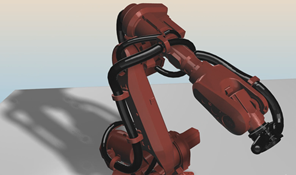
Fig. 16.3 Industrial robot with dresspack (cables) attached.

16.3. Creating a Cable

There are two parts to creating a cable: routing and properties configuration.

16.3.1. Routing

Cable routing is the process that defines the initial path of the cable. The user specifies the path using routing nodes. This section describe the default routing and segmentation algorithm, alternative algorithms are described in Direct segment routing and Path routing. A cable created from a collection of routing nodes will extend from node to node in the order that the nodes were added to the cable. Each such routing node pair is called a leg of the path. There are two types of routing nodes: FreeNode and BodyFixedNode. A FreeNode simply defines a location in space that the cable should pass through. This type of node produces no special behavior once the simulation has started.

agx::Real radius(0.05);
agx::Real resolution(3.35);
agxCable::CableRef cable = new agxCable::Cable(radius, resolution);
// Add 3 points in world coordinate system
cable->add(new agxCable::FreeNode(0.0, 0.0, 0.0));
cable->add(new agxCable::FreeNode(1.0, 0.5, 0.0));
cable->add(new agxCable::FreeNode(2.0, 0.3, 0.0));

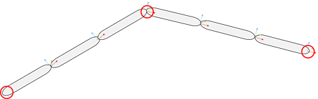
Fig. 16.4 Cable created from three FreeNodes indicated by red circles.

The points supplied defines the range of the cable in space, but does not include the capsule hemispheres. The cable will therefore be one cable diameter longer than the total distance between the routing nodes.

Fig. 16.5 Three cable segments created from three routing nodes.

The extra extent of the cable becomes important when an endpoint of the cable should be on the surface of some object. As shown in Fig. 16.6: Cable routed from the surface of a wall., placing the routing node on the surface will cause some initial overlap with the object. This will result in contacts and sudden cable movement when the simulation is started. Two possible solutions are to either place the routing node one cable radii away from the surface, or to disable collisions between the object and the first cable segment.

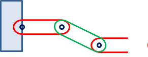
Fig. 16.6 Cable routed from the surface of a wall.

BodyFixedNodes are used to attach the cable to some other rigid body so the cable and the body will follow each other as the simulation progresses. The BodyFixedNode can be configured to either allow or prevent the body from rotating relative to the cable by providing different arguments to the BodyFixedNode constructor. By providing only an offset, in the form of an agx::Vec3, we specify that only that point on the body, in the body’s model coordinate frame, should be attached to the cable with a Ball Joint. By providing a full transformation, in the form of an agx::AffineMatrix4x4, we specify how the whole body should be placed relative to the cable using a LockJoint.

agx::RigidBodyRef rotatingBody = new agx::RigidBody();
agx::RigidBodyRef fixedBody = new agx::RigidBody();

// Attach the rotatingBody with a point: results in a BallJoint attachment constraint
cable->add(new agxCable::BodyFixedNode(rotatingBody, agx::Vec3()));

// Attach the rotatingBody with an AffineMatrix4x4: results in a LockJoint attachment constraint
cable->add(new agxCable::BodyFixedNode(fixedBody, agx::AffineMatrix4x4()));

When using a transformation matrix, the transformation describes where the routing node should be placed and how the body should be oriented relative to the cable, where the Z axis is defined to be along the cable.

Table 16.1 Cable routing node types.

Class	Description
agxCable::FreeNode	Initial positioning of cable.
agxCable::BodyFixedNode	Attach cable to rigid body.

The routing phase ends when the cable is added to a simulation. At this point the routing is finalized and segmentation is performed. Segmentation is the process that creates and positions segments between the routing nodes. The routing nodes are strictly adhered to, meaning that, except for at the cable end points, the routing node defines the end of one segment and the start of another. It is the responsibility of the segmentation algorithm to find a segment length that as evenly as possible divides all the route node pairs. This makes the smallest inter-node distance a lower bound on the cable’s resolution. The user supplied cable resolution is used as a start point for the search. It is not always possible to find a segment length that perfectly divides all path legs. In that case, some of the path legs will contain either small overlaps or small extra gaps. The intention is that these will be evened out during the first few time steps of the simulation. For this to work there must be some room for the cable to move. If two BodyFixedNodes are added next to each other then neither side can move and the cable may become unstable.

It is possible to dry-run the segmentation algorithm in order to gather information about the current routing without finalizing it. This is done by calling tryInitialize on the cable and returned is an initialization report that contains information such as the number of nodes created, the resolution of the cable, the largest segment error and the total length of the cable.

Additional routing nodes cannot be added to the cable after routing has been finalized. However, as an alternative to BodyFixedNodes the cable provides attachments that provide similar functionality. By attaching a rigid body to a cable segment the body will follow the cable as the simulation progresses. Attaching bodies this way follows the same translation/transformation rules as the BodyFixedNode. Note that adding attachments does not change the path of the cable, or the position of the attached object.

Attaching bodies requires a way to specify where along the cable the body should be attached. This is done using cable iterators, which are described in the Section 16.8.

agx::RigidBodyRef attachedBody = ...;
agxCable::CableIterator segment = ...;
// Attach a body with a BallJoint to the segment.
cable->attach(segment, attachedBody, agx::Vec3());

16.4. Direct segment routing

Direct segment routing is an an alternative to the segmentation process described in Section 16.3.1. Using direct segment routing it is possible to precisely control both the position and orientation of each individual cable segment during routing. This is useful when the cable path and segmentation is defined by an external tool or is known though some other means.

A cable with direct routing support is created by passing an instance of agxCable::IdentityRoute to the cable constructor instead of the resolution parameter. The routing nodes added to such a cable describe not only the path of the cable, but also the position and orientation of each and every segment. No additional segments will be created, and every segment will correspond to a routing node.

The transformation of the segments are configured by setting the transformation of the RigidBody that the routing node contains.

The segmentation algorithm handles the last routing node separately from the rest of the nodes. There is no such special handling when using direct segment routing. Just like every other segment, the last segment is placed with its start at the location of the corresponding routing node. When using the segmentation algorithm the last segment is placed with its end at the last routing node.

const agx::Real radius = agx::Real(0.04);
const agx::Real resolution = agx::Real(3.0);
agxCable::CableRef cable = new agxCable::Cable(radius, new agxCable::IdentityRoute(resolution));

agxCable::FreeNodeRef node1 = new agxCable::FreeNode(pos1);
node1->getRigidBody()->setRotation(rot1);
cable->add(node1);

agxCable::FreeNodeRef node2 = new agxCable::FreeNode(pos1);
node2->getRigidBody()->setRotation(rot2);
cable->add(node2);

agxCable::BodyFixedNodeRef node3 = new agxCable::BodyFixedNode(attachedBody, attachmentPointInBodyFrame);
node3->getRigidBody()->setPosition(pos3);
node3->getRigidBody()->setRotation(rot3);
cable->add(node3);

16.5. Path routing

Path routing is an alternative to the segmentation process described in Routing. Path routing work similarly to the default segmentation algorithm, but relaxes the requirements on individual segment placing. Instead of a sequence of routing legs the routing nodes are seen as a continuous path along which segments are placed.

16.6. Rebind

By default, a routed cable will try to straighten it self out, i.e. the resting state is a straight cable. But with the Cable::rebind() method, the current/initial state can become the resting state. Consider figure Fig. 16.7 where a cable is created as a spiral. By calling the rebind method, the current state of the cable will become the resting state. Any effort to straighten it out, will result in a restoration force to bring the cable back to its resting state. The example below is available as a python script in <agx-dir>/data/python/torsionSpiral.agxPy.

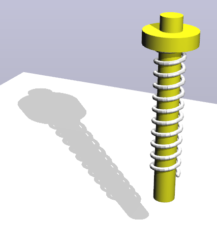
Fig. 16.7 Cable routed as a spiral using the rebind() method.

16.7. Properties

The cable provides several properties that control its behavior. These properties are accessed and modified via the agxCable::CableProperties class accessible using Cable::getCableProperties. Through the properties handle we can set things such as Young’s modulus and damping. Several cables can share the same properties handle, making it possible to easily configure and modify many cables at once.

Property name	Unit	Description
Young’s modulus	Pressure	Controls the stiffness of the cable.
Poisson’s ratio	unitless	Ratio of Stress over Strain. Will affect rotational stiffness when twisting.
Damping	Time	Controls how quickly potential energy in cable deformations dissipates.

The parameters can be set independently along the three dimensions of the cable: bend, twist and stretch. The following code snippet demonstrates how to set Young’s modulus in bend, twist and stretch directions.

agxCable::CableProperties* properties = cable->getCableProperties();
properties->setYoungsModulus(1e7, agxCable::BEND);
properties->setYoungsModulus(1e7, agxCable::TWIST);
properties->setYoungsModulus(1e7, agxCable::STRETCH);

Attention

Care should be taken when simulating cables with very low Young’s modulus in the stretch direction. The cable geometries are not resized when the cable is deformed leading to gaps in the cable during extreme elongation.

A different set of properties of the cable are those that all geometries have and that are represented by an instance of the agx::Material class. By assigning a material to a cable all geometries that make up that cable are assigned that same material. This, along with the contact materials created for the material assigned, control much of how the cable interacts with other objects in the scene. Some parameters share the same name as parameters found in the cable properties. Despite this, these are separate values with different purposes. For example, the Young’s modulus in the the geometry material control stiffness in contacts while the cable property with the same name control stiffness within the cable itself.

The density set in the geometry material is used to compute the mass of each cable segment, but due to the overlap between consecutive segments the total mass of the cable will be higher than what a density times volume computation would give. A higher resolution cable will have more segments and thus more overlaps and a larger mass discrepancy.

In addition to the internal damping in the cable, it is possible to set both linear and angular velocity damping of the cable using setLinearVelocityDamping and setAngularVelocityDamping.

16.7.1. Plasticity

A cable can be given plastic deformation properties by adding a CablePlasticity component to it. The plasticity parameters are configured on the CablePlasticity object using the same direction parameters as when configuring other direction dependent cable parameters.

agxCable::CableRef cable = ...;
agxCable::CablePlasticityRef plasticity = new CablePlasticity();
plasticity->setYieldPoint(1e9, agxCable::BEND);
cable->addComponent(plasticity);

The yield point specifies the torque required to permanently deform the cable, i.e., to cause a plastic deformation. Deformations in the stretch direction are always elastic.

16.8. Inspection using iterators

Some state of the cable, such as resolution and properties, apply to the whole cable while others, such as tension, vary along the cable. To inspect the latter the cable provides an iterator class that is used to iterate over the segments of the cable. Segmentation must have been performed on the cable before any iterators can be created. Using the iterator, we can find information such as the position of the segment, the rotational or translational tension and also get a hold of both the rigid body and the geometry that is used to represent the segment in the simulation.

for (agxCable::CableIterator segment = cable->begin();
!segment.isEnd();
++segment)
{
  // Use the accessor methods provided by CableIterator to inspect
  // dynamic cable state.
  agx::Real tension = segment->getStretchTension();
  agx::RigidBody* body = segment->getRigidBody();
  agxCollide::Geometry* geometry = segment->getGeometry();
}

The cable also supports range based for loops:

for (auto segment : *cable)
{
}

Once the cable has been initialized it is possible to create cable iterators directly from the routing nodes. This makes it possible to quickly get at the segment created near a particular node. This can be used, for example, to track the motion of some interesting point along the cable, or to find the geometry for a particular part of the cable in order to disable collisions between that geometry and geometries held by a body attached to the cable.

agxCable::CableRef cable = ...;
agx::RigidBodyRef body = ...;
agxCable::BodyFixedNodeRef node = new agxCable::BodyFixedNode(body, agx::Vec3());
cable->add(node);
simulation->add(cable);
agxCable::CableIterator segment(attachedNode);
agxUtil::setEnableCollisions(segment->getGeometry(), body, false);

A geometry, for example received as an argument to a contact event listener, can be passed to the static Cable::getCableForGeometry function and if that geometry is part of a cable then a pointer to that cable will be returned.

agxCollide::Geometry* geometry = ...;
// Return the Cable for which the geometry is part of. nullptr if the geometry is not
// part of any Cable.
agxCable::Cable* cable = agxCable::Cable::getCableForGeometry(geometry);

An initialized cable has two lengths: the rest length and the current length. The rest length is the sum och the lengths of the segments that make up the cable and the current length is the sum of the distances between the starting positions of consecutive segments, and the end position of the last segment. If there is no tension then the two lengths are the same, but if there is some load on the cable then the two lengths may differ. We say that the cable has become either stretched or compressed. The amount of stretch a given load produces is controlled by configuring Young’s modulus on the cable.

16.9. Hydro- and aerodynamics

A cable is affected by the fluid that surrounds it. A WindAndWaterController can be used to simulate the affects in water, air and other fluids, see Section 22.

16.10. Known limitations

• Mass not properly computed from density because of hemisphere overlaps.

• Geometries are not resized to match the current stretching of the cable.

• Cables must be circular.

• Cables must be homogeneous, both in size and properties.