19. AGX DriveTrain

AGX DriveTrain is a library within the AGX PowerLine framework designed to model the various components of a vehicle’s drivetrain. It focuses exclusively on the rotational motion, meaning that all its components inherit from either RotationalUnit or RotationalConnector.

The following C++ example demonstrates how to build a simple AGX DriveTrain system using the AGX PowerLine framework.

// Create a ``PowerLine`` instance that will hold all drivetrain components
agxPowerLine::PowerLineRef powerLine = new agxPowerLine::PowerLine();
simulation->add(powerLine);

// Initialize an engine using predefined library parameters (e.g., Saab B234i).
agxDriveTrain::CombustionEngineParameters engineParameters;
agxDriveTrain::CombustionEngine::readLibraryProperties("Saab-B234i", engineParameters);
agxDriveTrain::CombustionEngineRef engine = new agxDriveTrain::CombustionEngine(engineParameters);
powerLine->add(engine);

// Create a simple shaft to transmit torque between engine and torque converter.
agxDriveTrain::ShaftRef engineShaft = new agxDriveTrain::Shaft();
powerLine->add(engineShaft);

// Add a torque converter to simulate automatic transmission behavior.
agxDriveTrain::TorqueConverterRef torqueConverter = new agxDriveTrain::TorqueConverter();
powerLine->add(torqueConverter);

// Create a shaft to transmit torque between torque converter and gear.
agxDriveTrain::ShaftRef torqueConverterShaft = new agxDriveTrain::Shaft();
powerLine->add(torqueConverterShaft);

// Add a gear component to model the transmission ratio.
agxDriveTrain::GearRef gear = new agxDriveTrain::Gear();
powerLine->add(gear);

// Create a shaft to transmit torque between gear and differential.
agxDriveTrain::ShaftRef gearShaft = new agxDriveTrain::Shaft();
powerLine->add(gearShaft);

// Add a differential to distribute torque between wheels.
agxDriveTrain::DifferentialRef differential = new agxDriveTrain::Differential();
powerLine->add(differential);

// Connect the differential to the wheel actuator (linked to a hinge joint in the scene).
agxPowerLine::RotationalActuatorRef wheelActuator = new agxPowerLine::RotationalActuator(hinge);
powerLine->add(wheelActuator);

// Connect all drivetrain components in sequence.
engine->connect(engineShaft);
engineShaft->connect(torqueConverter);
torqueConverter->connect(torqueConverterShaft);
torqueConverterShaft->connect(gear);
gear->connect(gearShaft);
gearShaft->connect(differential);
differntial->connect(wheelActuator);

Note

• Ensure that each component is added to the same PowerLine instance before connecting them.

• Component order should reflect the actual power flow — from engine → wheels.

• A detailed description of each drivetrain component is provided in the subsequent sections.

19.1. Engines

An engine is a type of RotationalUnit that serves as the primary source of power within a drivetrain system. AGX DriveTrain provides three types of engines:

• Combustion engine: A conventional power source that converts fuel energy into rotational motion.

• Torque curve based engine: Uses a predefined torque-speed relationship.

• Fixed velocity engine: Maintains a constant output speed regardless of load.

Each type has distinct modeling characteristics depending on the simulation’s goals and desired level of physical realism.

19.1.1. Combustion engine

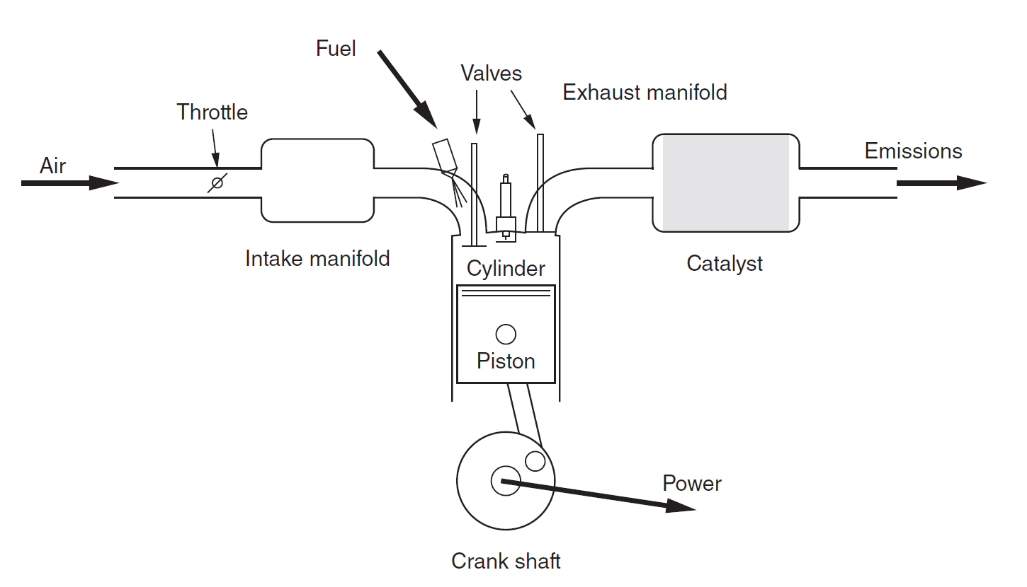
The Combustion engine [13] is one of the most commonly used power source in vehicles, excavators, wheelloaders, aircraft, and marine propulsion systems. It consists of several key components (see Fig. 19.1), including

• Cylinders and Pistons: The main body of the engine where combustion occurs.

• Crankshaft and Camshafts: Convert the pistons’ linear motion into rotational motion, transmitting power to the drivetrain;

• Valves: Control the intake and exhaust flow.

• Fuel Injection and Ignition Systems: Regulate and initiate the combustion process.

• Air Intake and Exhaust Systems: Manage airflow and remove combustion gases.

Fig. 19.1 Combustion engine schematic (source: [13]).

As a critical component of the vehicle, the combustion engine plays a decisive role in the vehicle’s dynamic performance, including stability, handling, and ride comfort. A well-modeled engine provides valuable data such as:

• Engine speed

• Torque

• Power

• Fuel consumption

These outputs are essential for designing efficient powertrain systems and developing effective vehicle control strategies, meeting the increasing demands for accurate and efficient simulations.

Modelling of the combustion engine involves applying mathematical equations that describe its physical behavior, including:

• Thermodynamics: Determines engine efficiency and power output.

• Fluid Mechanics: Governs airflow and fuel delivery to the combustion chamber.

• Rotational Dynamics: Represents the crankshaft, connecting rods, and their conversion of linear piston motion into rotational motion.

19.1.1.1. Modelling theory

In AGX Dynamics, the mean value engine model (MVEM) [13] is implemented to represent the combustion engine. MVEM is a simplified, time-based model that predicts averaged engine combustion variables without simulating the detailed in-cylinder combustion process. It captures the dominant combustion characteristics averaged over one or several engine cycles.

The governing equations of the MVEM are two ordinary differential equations as shown below.

\[\begin{split}\frac{d\!{\ p_{\text{im}}}}{d\!{\ t}} & = \frac{RT_{\text{im}}}{V_{\text{im}}}(\dot{m}_{\text{at}} - \dot{m}_{\text{ac}}) \\ \mathcal{J}\frac{d\!{\ N}}{d\!{\ t}} & = M_{i} - M_{f} - M_{p} - M_{load}\end{split}\]

The first equation describes the development of the intake manifold pressure \(p_{\text{im}}\). Here, \(T_ {\text{im}}\) is the intake temperature, \(V_{im}\) is the intake manifold volume, and \(R\) is the specific gas constant. The difference between throttle inflow \(\dot{m}_{\text{at}}\) and cylinder outflow \(\dot{m}_{\text{ac}}\) determines the rate of mass change in the intake system. This equation is derived from the ideal gas law \(pV = mRT\).

The second equation governs the rotational dynamics of the engine crankshaft, with the moment of inertia \(J\). \(N\) is the rotational speed of the crank shaft, \(M_i\) is the indicated torque, \(M_f\) is the internal friction torque, \(M_{p}\) is the pumping torque, \(M_{load}\) is the output(load) torque.

19.1.1.1.1. Throttle mass flow

The throttle air mass flow \(\dot{m}_{at}\), depends not only on the throttle plate position but also on the intake manifold pressure. It can be expressed as [6],

\[\begin{split}\dot{m}_{\text{at}} & = \frac{p_{\text{amb}}}{\sqrt{RT_{\text{amb}}}}A_{\text{eff}}(\alpha) \Psi_{\text{li}} \left( \Pi \left( \frac{p_{\text{im}}}{p_{\text{amb}}} \right) \right) \\\end{split}\]

where \(T_{\text{amb}}\) and \(p_{\text{amb}}\) are the ambient temperature and pressure, respectively. \(A_{\text{eff}}(\alpha)\) is the effective throttle openning area, and \({\Psi_{\text{li}} \left( \Pi \left( \frac{p_{\text{im}}}{p_{\text{amb}}} \right) \right)}\) is the flow function. Due to the large pressure difference across the throttle, the airflow velocity can reach 70–100 m/s. This flow is modeled as isentropic compressible flow.

19.1.1.1.2. Engine mass flow

The cylinder air mass flow \(\dot{m}_{ac}\) depends on the engine speed \(N\), intake pressure \(p_{\text{im}}\), and temperature \(T_{\text{im}}\). It is defined as,

\[\begin{split}\dot{m}_{\text{ac}} & = \nu_{\text{vol}}(N,p_{\text{im}},\ldots)\frac{V_{D}Np_{\text{im}}}{n_{r}RT_{\text{im}}} \\\end{split}\]

where \(\nu_{vol}\) is the volumetric efficiency, which represents the engine’s ability to draw fresh air into the cylinders. It can be modeled as [14]

\[\begin{split}\nu_{\text{vol}} & = c_{0} + c_{1}N + c_{2}N^2 + c_{3}p_{\text{im}}\\\end{split}\]

Here, \(c_{0}\), \(c_{1}\), \(c_{2}\), \(c_{3}\) are pressure- and engine-speed-dependent coefficients.

19.1.1.1.3. Engine torques

The engine torques – indicated torque \(M_{i}\), friction torque \(M_f\), and pump torque \(M_p\) – are calculated as

\[\begin{split}M_{i} & = \frac{\dot{m}_{f}Q_{hv}\eta_{t}}{N} = \frac{\dot{m}_{ac}Q_{hv}\eta_{t}}{AF \cdot N} \\ M_{f} & = \frac{V_{D}}{2\pi{n_{r}}} \left(C_{fr0} + C_{fr1}\frac{N}{1000} + C_{fr2}\left(\frac{N}{1000}\right)^2\right)\\ M_{p} & = \frac{V_{D}}{2\pi{n_{r}}}(p_{em} - p_{im}) \\\end{split}\]

where

• \(\dot{m}_{f}\)– fuel flow rate

• \(Q_{hv}\) – fuel heat value

• \(\eta_{t}\)– thermal efficiency

• \(AF\) – stoichiometric air-fuel ratio

• \(C_{fr0}\), \(C_{fr1}\), \(C_{fr2}\) – friction torque coefficients [13]

• \(p_{em}\) – exhaust manifold pressure

Note

The default friction coefficients – \(C_{fr0} = 0.97\), \(C_{fr1} = 0.15\) and \(C_{fr2} = 0.04\) – are suggested as representative values for engines with displacement volumes between 0.845L and 2.0L [13]. For other engines outside this range, these parameters should be calibrated against real engine test data.

19.1.1.2. Build combustion engine

The combustion engine can be parameterized, created and initialized as shown below:

// Initialize the engine as a Saab B234i engine.
agxDriveTrain::CombustionEngineParameters engineParameters;
agxDriveTrain::CombustionEngine::readLibraryProperties("Saab-B234i", engineParameters);
agxDriveTrain::CombustionEngineRef engine = new agxDriveTrain::CombustionEngine(engineParameters);

// Enable the engine before it can start.
engine->setEnable(true);

In this example, the Saab B234i engine configuration is used, which has a 2.3-liter displacement volume and delivers a maximum torque of 212 Nm at 4000 RPM.

An engine can also be reconfigured after creation:

// Assume that the engine has been initialized as a Saab B234i engine.
// Reconfigure it as a Volvo T5.
engine->loadLibraryProperties("Volvo-T5");
engine->setEnable(true);

19.1.1.2.1. Engine Parameters

The AGX Dynamics data directory includes a set of predefined engine models stored in JSON format. These files are located at: <agx_dir>/data/MaterialLibrary/CombustionEngineParameters.

Each file contains a parameter set (e.g., “Saab-B234i”, “Scania-K310UB4X2Euro5”) and the corresponding torque-friction coefficients. You can define a new engine model by copying an existing file and modifying the parameters as needed. Alternatively, parameters can be set explicitly in code:

agxDriveTrain::CombustionEngineParameters engineParameters;
engineParameters.displacementVolume = 0.003;
engineParameters.maxTorque = 300;
engineParameters.maxTorqueRPM = 3000;
engineParameters.maxPowerRPM = 4000;
engineParameters.idleRPM = 1000;
engineParameters.maxRPM = 9000;
engineParameters.crankShaftInertia = 0.5;
agxDriveTrain::CombustionEngineRef engine = new agxDriveTrain::CombustionEngine(engineParameters);
engine->setEnable(true);

The following table lists all available parameters for customizing a combustion engine:

Parameter	Unit	Description
displacementVolume	m^3	Total cylinder displacement volume of the engine.
maxTorque	Nm	Maximum rated torque the engine can produce over short or continuous operation.
maxTorqueRPM	RPM	Crankshaft speed at which maximum torque is achieved.
maxPowerRPM	RPM	Crankshaft speed at which maximum power is produced.
idleRPM	RPM	Crankshaft speed under idle conditions.
maxRPM	RPM	Maximum allowable crankshaft speed.
crankShaftInertia	kg m^2	Moment of inertia of the crankshaft.
cfr0		Coefficient defining the quadratic relationship between friction torque and engine speed.
cfr1		Coefficient defining the quadratic relationship between friction torque and engine speed.
cfr2		Coefficient defining the quadratic relationship between friction torque and engine speed.
throttlePinBoreRatio		Ratio between throttle pin and bore diameters (optional)
maxVolumetricEfficiency		Maximum volumetric efficiency; ratio of actual air intake volume to swept cylinder volume (optional).
airFuelRatio		Stoichiometric air–fuel ratio for complete combustion (optional).
heatValue	J/kg	Heat value of the fuel (optional).
nrRevolutionsPerCycle		Number of revolutions per cycle, e.g., RevolutionsPerCycle::TWO_STROKE or RevolutionsPerCycle::FOUR_STROKE

19.1.1.2.2. Throttle control

The engine’s behaviour can be controlled via the throttle input. The throttle value ranges from 0 (idle) to 1 (fully open):

engine->setThrottle(throttle);

The available throttle-related parameters and methods are listed below:

Parameter	Method	Description
Throttle	setThrottle	Sets the throttle opening as a percentage between 0 (fully closed) and 1 (fully open).
Throttle Angle	setThrottleAngle	Defines the throttle plate position directly in radians rather than as a percentage.
Idle Throttle Angle	setIdleThrottleAngle	Specifies the minimum throttle plate angle when the engine is idling.
Max. Throttle Angle	setMaxThrottleAngle	Limits the maximum throttle plate angle during full throttle operation.

Additional engine settings, such as the number of revolutions per cycle and other configuration details, can also be adjusted to match specific engine types or performance requirements.

Detailed C++ and Python examples can be found in:

• <agx_dir>/tutorials/tutorial_driveTrain_combustionEngine.cpp

• <agx_dir>/data/python/tutorials/tutorial_driveTrain_combustionEngine.agxPy

• <agx_dir>/data/python/tutorials/tutorial_driveTrain_torque_converter.agxPy

19.1.1.3. Engine performance

Fig. 19.2 shows the torque and power curves for the Saab engine configuration. Both simulated and measured results are included to demonstrate and verify the correspondence between the model predictions and experimental data.

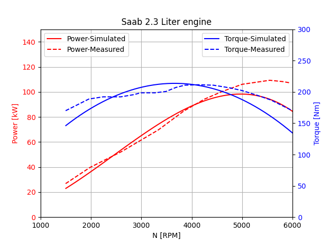
Fig. 19.2 Torque and power curves of Saab engine.

Fig. 19.3 illustrates the performance of the Volvo excavator engine. Similar to the Saab case, the figure compares simulated and measured data to validate the model’s ability to reproduce the engine’s real-world behavior.

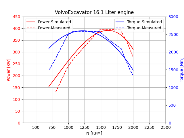
Fig. 19.3 Torque and power curves of the Volvo excavator engine.

19.1.2. Torque curve based engine

A torque curve based engine determines its output torque based on a predefined torque–speed relationship. It uses a torque curve to find the maximum available torque at the current engine speed (RPM), and a user-controlled throttle to scale that torque proportionally.

19.1.2.1. Example usage

A typical setup looks like this:

// Create an Engine instance.
agxDriveTrain::EngineRef engine = new agxDriveTrain::Engine();

// Access the engine’s internal torque curve lookup table.
// This table defines how much torque the engine delivers at different speeds (RPM).
agxPowerLine::PowerGenerator* powerGenerator = engine->getPowerGenerator( );
agxPowerLine::PowerTimeIntegralLookupTable* torqueCurve = powerGenerator->getPowerTimeIntegralLookupTable();

// Insert torque–speed data points into the lookup table.
// Each pair (rpmX, torqueX) represents the engine’s torque output at a given engine speed.
torqueCurve->insertValue(rpm0, torque0);
torqueCurve->insertValue(rpm1, torque1);
torqueCurve->insertValue(rpmN, torqueN);

// Set the throttle input that controls the engine’s behavior (e.g., power output).
engine->setThrottle(throttle);

At each simulation step, the engine performs a lookup in the torque curve table to find the maximum available torque for the current RPM. It then multiplies this value by the current throttle (a scalar between 0 and 1) to determine the effective torque applied during that step.

The lookup table uses piecewise linear interpolation between inserted data points and linear extrapolation using the first or last two points when the RPM is outside the defined range.

An Engine also defines an idle RPM, along with a corresponding minimum torque value in its power generator. When the engine speed falls below the idle RPM, the generator applies at least this minimum torque to bring the engine back up to its idle speed.

19.1.2.2. PID-controlled engine

A variant of the torque curve based engine is the PidControlledEngine, which extends Engine with additional control capabilities.

It behaves similarly by default, but adds:

• Ignition control — start and stop the engine programmatically.

• Automatic throttle control — maintain a target RPM or implement custom throttle strategies.

Automatic throttle control is implemented via a ThrottleCalculator interface. The built-in RpmController is a PID-based implementation that regulates throttle input to maintain a desired RPM target.

engine = new agxDriveTrain::PidControlledEngine();

// Create and assign the engine’s torque curve before enabling ignition.
agxPowerLine::PowerGenerator* powerGenerator = engine->getPowerGenerator( );
agxPowerLine::LookupTable* torqueCurve = powerGenerator->getPowerTimeIntegralLookupTable( );
torqueCurve->insertValue(rpm0, torque0);
torqueCurve->insertValue(rpm1, torque1);
torqueCurve->insertValue(rpmN, torqueN);

// Create an RPM controller that regulates the engine’s throttle to maintain a target RPM.
// The PID gains (pGain, iGain, dGain) determine the control response, and iRange limits the integral term.
controller = new agxDriveTrain::RpmController(engine, targetRpm, pGain, dGain, iGain, iRange);

// Assign the controller to the engine’s throttle calculator.
// This allows the engine’s throttle to be automatically adjusted based on the PID control logic.
engine->setThrottleCalculator(controller);

// Enable the engine ignition to start the power generation process.
engine->ignition(true);

Here, it is worth noting that the idle control in a PidControlledEngine differs conceptually from that of the base Engine (which relies purely on a torque curve):

• When a ThrottleCalculator (such as RpmController) is assigned, it takes full control of the throttle to maintain the target RPM — including idle conditions.

• When no controller is set, the engine automatically adjusts torque using setGradient to reach and sustain its idle RPM.

19.1.3. Fixed velocity engine

Unlike combustion- or lookup-based engines, which calculate torque based on physical or empirical relationships, a fixed velocity engine imposes motion directly.

19.1.3.1. Principle of operation

The fixed velocity engine maintains a constant rotational speed by enforcing a velocity constraint on its output shaft.

\[0 = \omega_{e}-\omega_{0} + \epsilon \tau\]

where \(\omega_{e}\) refers to the angular speed of the engine output shaft, \(\omega_{0}\) is the target velocity, \(\tau\) is the torque transfer bounded within \([-\infty,\infty]\), and \(\epsilon\) is the regularization parameter of the velocity constraint.

Functionally, the fixed velocity engine behaves as an idealized actuator with effectively unlimited torque capacity. It instantly compensates for load variations or transient disturbances to maintain the prescribed speed.

Since torque is derived implicitly from the velocity constraint, the model excludes combustion, throttle control, and frictional effects. Its simplicity and determinism make it particularly useful for drivetrain validation, mechanical subsystem studies, and other cases where a constant input speed is required.

This approach guarantees a perfectly constant shaft velocity over time, making the model well-suited for testing, debugging, and validating drivetrain components under controlled input conditions.

19.1.3.2. Example usage

// Create a fixed velocity engine

agxDriveTrain::FixedVelocityEngineRef engine = new agxDriveTrain::FixedVelocityEngine();

// Set the target angular velocity (in radians per second)
engine->setTargetVelocity(100.0);
engine->setEnable(true);

This setup will maintain the output shaft velocity at 100 rad/s, independent of external load or resistance in the drivetrain.

19.2. ElectricMotor

An ElectricMotor is a type of Unit that, like an engine, acts as a source of power within a drivetrain. It models the conversion of electrical energy to mechanical energy, producing torque that drives the connected shaft.

19.2.1. Physical model

The behavior of the electric motor is defined by its resistance, inductance, torque constant, and back electromotive force (EMF) constant. These parameters describe how the motor responds to voltage and current, and how it converts electrical input into rotational motion.

The torque constant, \(\alpha\), defines the proportional relationship between the motor torque \(\tau\), and the current, \(I\) flowing through the windings:

\[\tau = \alpha I.\]

The back EMF constant, denoted \(\beta\), defines the proportional relationship between the back EMF \(V\), and the angular velocity \(\omega\) of the rotor,

\[V = \beta \omega.\]

For an ideal motor, the constants are equal, \(\alpha = \beta\). In practical systems, however, energy losses (primarily due to resistive heating in the armature) reduce efficiency, leading to \(\beta \leq \alpha\). These losses become more significant at high current, where a portion of the electrical input energy is dissipated as heat rather than converted to mechanical work.

19.2.2. Example usage

When an ElectricMotor is created, the input voltage is initialized to zero. To start the motor, a nonzero voltage must be applied.

agxDriveTrain::ElectricMotorRef motor = new agxDriveTrain::ElectricMotor( resistance, torqueConstant,
                                                                          emfConstant, inductance );
motor->setVoltage( voltage );

The applied voltage can be updated at each simulation step, allowing the user to regulate the angular velocity or torque output of the motor in real time. This can be typically done by implementing a control system (for example, a PID controller) that adjusts the input voltage based on measured speed or torque targets.

Note

• Ensure the chosen constants accurately represent the physical motor being simulated. Incorrect values can cause unrealistic response or numerical instability.

• The motor can be integrated with other Unit such as gearboxes or clutches to build complete electric drive systems.

19.3. Shaft

A Shaft is a fundamental drivetrain Unit representing a rotating mechanical element that transmits torque and angular velocity between connected components in the power line.

As the rotational equivalent of a mechanical link, it forms the system’s backbone, connecting components like engine, clutch, torque converter, and gearbox.

19.3.1. Example usage

agxDriveTrain::ShaftRef shaft1 = new agxDriveTrain::Shaft();
powerLine->add(shaft1);

engine->connect(shaft1);
shaft1->connect(clutch);

This example creates a new shaft and adds it to an existing AGX PowerLine. Once added, the shaft can be connected to other components such as engine, clutch, or gearbox through its connect methods.

19.3.2. Rotational Inertia

Each shaft possesses a physical property – rotational inertia – defines the resistance of the shaft to angular acceleration. It can rotate freely unless constrained by connected units. By default, a shaft has a rotational inertia determined by its assigned moment of inertia, which can be set explicitly to control how quickly it accelerates under torque:

shaft1->setInertia(0.25); // kg·m²

A larger inertia results in smoother, slower acceleration, while a smaller value makes the system respond more quickly to torque changes.

19.4. TorqueConverter

A torque converter is a critical component in an automatic transmission system. It consists of three main mechanical elements: the pump impeller, stator, and turbine runner, as illustrated in Fig. 19.4.

Fig. 19.4 Torque converter schematic [15].

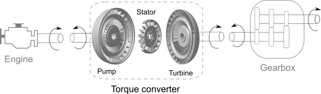
The torque converter transfers rotational power from the engine to the transmission via fluid. The impeller, driven by the engine, accelerates the transmission fluid toward the turbine. The turbine then converts the fluid’s momentum into mechanical torque, while the stator redirects the returning fluid to enhance torque multiplication and overall efficiency.

Functionally, the torque converter serves a role similar to that of a clutch in a manual transmission system. However, unlike a clutch — which disconnects the engine from the transmission when the vehicle stops — the torque converter allows the engine to continue spinning independently of the transmission. This enables the vehicle to remain stationary without stalling the engine.

19.4.1. Modelling strategy

In AGX Dynamics, the torque converter is modeled as such a viscous coupling between two rotating shafts, implemented through a look-up table-based model. When there is a velocity difference between the input and output shafts, the torque converter produces torque multiplication. This approach offers low computational cost and relies primarily on measured data, making it efficient and suitable for real-time simulation. It provides practical accuracy without the complexity or parameter sensitivity of dynamic or CFD-based models.

The performance of a torque converter depends on the internal design of its pump and turbine. Two key characteristic tables define its behavior:

• Geometry Factor Table

• Efficiency Table

The geometry factor, denoted as \(\xi(\nu)\), is a function of the velocity ratio \(\nu = \omega_t / \omega_p\) (the ratio of turbine to pump angular velocity). It is used to calculate the torque required to drive the pump:

\[M_{p} = \xi(\nu) \rho d_{p}^{5} \omega_{p}^{2},\]

where

• \(\rho\) – fluid density

• \(d_{p}\) – pump diameter

The efficiency, denoted as \(\psi(\nu)\), defines the ratio of the turbine torque to the pump torque. The turbine torque \(M_{t}\) is derived from the pump torque as:

\[M_{t} = \psi(\nu) M_{p},\]

This relationship describes how effectively the torque converter transfers energy between its components. The above-mentioned parameters can be adjusted to tune the torque converter’s overall behavior.

19.4.2. Example usage

A torque converter can be created and added to a drivetrain as follows:

// Create a torque converter and attach it to the power line.
agxDriveTrain::TorqueConverterRef tc = new TorqueConverter();
powerLine->add(tc);

// Configure the geometry factor table, defining the relationship
// between the velocity ratio and the pump torque scaling.
TorqueConverter::setGeometryFactorTable(const agx::RealPairVector& velRatio_geometryFactor);

// Configure the efficiency table, defining how effectively the turbine
// transfers torque relative to the pump across different velocity ratios.
TorqueConverter::setEfficiencyTable(const agx::RealPairVector& velRatio_efficiency);

// The torque converter also includes a lock-up mechanism that can synchronize
// the input and output velocities for improved efficiency during steady driving conditions.
tc->enableLockUp(true);

By default, the torque converter is initialized with generic parameters suitable for typical use. It can be connected directly to the drivetrain and used without additional configuration.

Detailed C++ and Python examples with torque converter are available in

• <agx_dir>/tutorials/tutorial_driveTrain.cpp and

• <agx_dir>/data/python/tutorials/tutorial_driveTrain_torque_converter.agxPy

Note

• For more advanced applications, the geometry factor and efficiency tables can be customized to achieve specific performance characteristics or to replicate measured converter data.

• Fine-tuning of parameters ensures stable, realistic, and efficient drivetrain performance.

19.5. DryClutch

The dry-clutch, as shown in Fig. 19.5 a), is a mechanism that enables the engine to be connected to or disconnected from the rest of the transmission system without stalling the engine. This is achieved by pressing friction plates against each other, allowing controlled slip during the engagement phase.

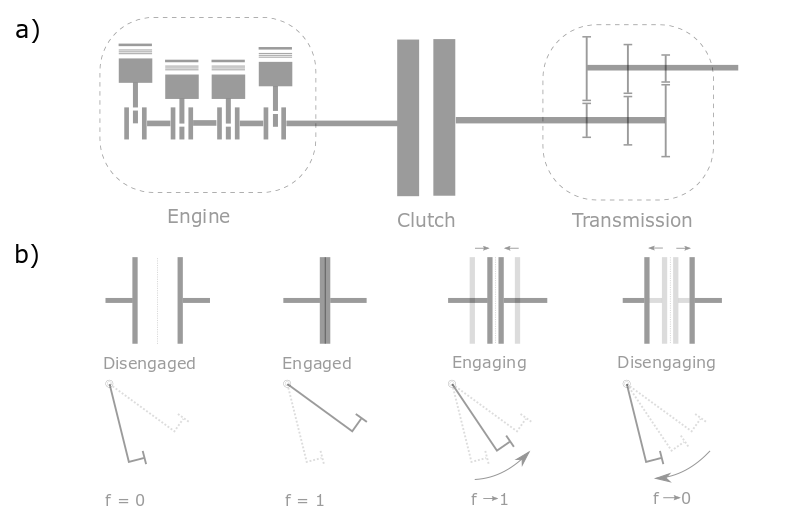
Fig. 19.5 Dry clutch schematic. a) Relative position; b) Working schemes.

Fig. 19.5 b) shows the operational principles of the clutch. A variable of fraction, denoted as \(f\), represents the relative position of the clutch discs corresponding to the clutch pedal operation. When \(f = 0\), the clutch is fully disengaged, meaning the clutch pedal is fully depressed. Conversely, \(f = 1\) indicates a fully engaged clutch. During the engagement and disengagement process, \(f\) varies continuously within the range \([0, 1]\).

19.5.1. Governing equations

The dry-clutch is modelled based on dry friction between input and output shafts, combined with a locking mechanism that engages when the two shafts rotate at nearly the same angular velocity. Dry friction is represented as a velocity (nonholonomic) constraint which enforces that the relative velocities of the connected shafts remain equal as long as the torque required to maintain this condition stays below the slip threshold.

\[0 = \omega_{e}-\omega_{s} \perp \tau \in[-\tau_{C},\tau_{C}]\]

where \(\omega_{e}\) denotes the angular speed of the engine crackshaft, \(\omega_{s}\) is the angular speed of the transmission input shaft, \(\tau\) represents the torque transmitted through the clutch discs, \(\tau_{C}\) is the maximum torque capacity of the clutch.

The perpendicularity condition \(\perp\) indicates a complementarity relationship between the relative angular velocity and the transmitted torque. This means that:

• if \(\omega_{e}-\omega_{s} = 0\) then \(-\tau_{C} < \tau < \tau_{C}\) (no slip),

• if \(\omega_{e}-\omega_{s} > 0\) then \(\tau = -\tau_{C}\), and

• if \(\omega_{e}-\omega_{s} < 0\) then \(\tau = \tau_{C}\).

When the lock (a positional, or holonomic constraint) is activated, the following condition is imposed:

\[0 = \phi_{e}-\phi_{s}\]

where \(\phi_{e}\) denotes the angular position of the engine crackshaft, \(\phi_{s}\) is the angular position of the transmission input shaft.

This constraint models the clutch’s locking mechanism, ensuring the engine crackshaft and the transmission input shaft rotate as a single rigid body. In the locked state, there are no limits on the transmitted torque, as the connection is fully rigid.

19.5.2. Parameters

As described above, the dry clutch model involves several physical parameters – such as the torque capacity and engagement fraction – used for both modelling and simulation. In addition, a number of simulation control parameters must be specified by the user, as listed in the table below.

Parameter	Method	Description	Default
\(f\)	setFraction	Fraction of the maximum distance between the clutch plates (or equivalently, the fraction of the maximum normal force between the clutch pads and the flywheel). The value varies between 0 and 1.	0
\(\tau_{C}\)	setTorqueCapacity	Maximum torque transferable through the clutch plates (in N·m)	225
autoLock	setAutoLock	Enables or disables the auto locking feature	False
engageTimeConstant	setEngageTimeConstant	Time constant governing the transition from the disengaged to the engaged state. Its unit is consistent with the simulation time step. The time constant ranges within \((0, \infty]\), where \(\infty\) indicates that the clutch pedal remains fixed in its current position.	2.5
disengageTimeConstant	setDisengageTimeConstant	Time constant governing the transition from the engaged to the disengaged state.	1.0
minRelativeSlip	setMinRelativeSlip	Threshold used to determine whether the locking criterion is satisfied. The parameter is dimensionless	1e-5
manual	setManualMode	Set the clutch control mode: manual or automatic (See Clutch manipulation)	False
engage	setEngage	Activate clutch engagement (True) or disengagement (False)	False

The default values of torque capacity \(\tau_{C}\) and the time constants are adopted from [5], which correspond to the engine of a medium size passenger car. For heavy duty engine, the clutch torque capacity can reach up to 1200N·m [6].

It is worth noting that all the parameters are fully customizable. Users can adjust them to reflect different clutch characteristics or to simulate varying driving conditions and operational scenarios, such as traffic-dependent behavior.

19.5.3. Build clutch

The clutch is constructed, configured and connected as follows:

// Create a power line to host drivetrain components.
agxPowerLine::PowerLineRef powerLine = new agxPowerLine::PowerLine();

// Create the dry clutch and set key physical/simulation parameters.
agxDriveTrain::DryClutchRef dryClutch = new agxDriveTrain::DryClutch();
dryClutch->setTorqueCapacity(400.0);
dryClutch->setEngageTimeConstant(2.5);
dryClutch->setDisengageTimeConstant(1.0);
dryClutch->setAutoLock(true);

// Add the clutch to the power line.
powerLine->add(dryClutch);

// Create an engine and a transmission-side shaft, then connect them via the clutch.
agxDriveTrain::FixedVelocityEngineRef engine = new agxDriveTrain::FixedVelocityEngine();
agxDriveTrain::ShaftRef transmissionShaft = new agxDriveTrain::Shaft();

// Connect engine to the input side of the clutch and the output side to the transmission.
dryClutch->connect(engine);
dryClutch->connect(transmissionShaft);

Once the clutch is built, it can be connected to the engine (See Engines) and transmission shafts (See Shaft).

19.5.4. Clutch manipulation

The clutch supports two control modes: manual and automatic:

• In manual mode, the user drives the engagement directly via setFraction() with a value in \([0,1]\).

• In automatic mode, the user toggles engagement with setEngage(bool), while the time constants govern the ramp behavior.

Manual mode example – gradually engage over 1 s, then linearly disengage over 2 s:

class ManualClutchListener : public agxSDK::StepEventListener
{
public:
  // Constructor: takes a pointer to the DryClutch instance
  ManualClutchListener(agxDriveTrain::DryClutch* clutch) :
  m_clutch(clutch)
  {
    // Ensure the clutch is in manual mode so setFraction() is honored.
    m_clutch->setManualMode(true);
  }
  void pre(const agx::TimeStamp& t)
  {
    // Example schedule:
    // 0–1 s   : ramp fraction from 0 -> 1 (engaging)
    // 1–3 s   : ramp fraction from 1 -> 0 (disengaging)
    if (t > 0 && t <= 1.0) {
      m_clutch->setFraction(t); // linearly 0 -> 1 over 1 s
    }
    else if (t > 1.0 && t <= 3.0) {
      m_clutch->setFraction(1 - (t-1) / 2);  // 1 -> 0 over 2 s
    }
private:
  agxDriveTrain::DryClutch* m_clutch = nullptr;
}

Automatic mode example — use setEngage() with time constants:

class AutoClutchListener : public agxSDK::StepEventListener
{
  public:
    AutoClutchListener(agxDriveTrain::DryClutch* clutch) :
    m_clutch(clutch)
    {
      // Ensure automatic mode so setEngage() is effective.
      m_clutch->setManualMode(false);
    }
    void pre(const agx::TimeStamp& t)
    {
      // Example schedule:
      // 3–5 s   : engage over 2 s
      // 7–9 s   : disengage over 1 s
      // else    : hold current state (infinite time constants)
      if (t > 3.0 && t <= 5.0)
      {
        m_clutch->setEngage(true);
        m_clutch->setEngageTimeConstant(2.0);     // 0 -> 1 in 2 s
      }
      else if (t> 7.0 && t <= 9.0)
      {
        m_clutch->setEngage(false);
        m_clutch->setDisengageTimeConstant(1.0); // 1 -> 0 in 1 s
      }
      else {
        // "Hold" behavior: changes are effectively frozen.
        m_clutch->setEngageTimeConstant(agx::Infinity );
        m_clutch->setDisengageTimeConstant(agx::Infinity);
      }
  private:
    agxDriveTrain::DryClutch* m_clutch = nullptr;
  }

Detailed C++ and Python examples with DryClutch are available in

• <agx_dir>/tutorials/tutorial_driveTrain.cpp and

• <agx_dir>/data/python/tutorials/tutorial_driveTrain_dryClutch.agxPy.

Note

• Use setManualMode(true) when driving setFraction().

• Use setManualMode(false) when driving setEngage().

• The “hold” behavior is achieved by setting time constants to infinity, which maintains the current state.

19.6. Gear

The Gear is the most fundamental drive train Connector. It transfers rotational motion between the Unit-based drive train components. A Gear represents the interaction between two geared wheels – one on each connected Unit – and is characterized by a gear ratio.

The gear ratio defines the number of gear teeth on the output shaft relative to the input shaft.

• A gear ratio greater than 1 causes the output gear to rotate slower than the input,

• A gear ratio less than 1 makes the output gear rotate faster than the input shaft,

• A negative ratio reverses the rotation direction of the output shaft.

Mathematically:

\[\omega_{out} = \frac{\omega_{in}}{g}\]

where \(g\) is the gear ratio.

A pair of shafts can be connected with the gear using the following example code:

agxDriveTrain::ShaftRef inputShaft = new agxDriveTrain::Shaft();
agxDriveTrain::ShaftRef outputShaft = new agxDriveTrain::Shaft();

// Create a reference to a new gear that will connect the two shafts
agxDriveTrain::GearRef gear = new agxDriveTrain::Gear();

// Add the created components to the power line system
powerLine->add(inputShaft);
powerLine->add(outputShaft);
powerLine->add(gear);

// Set the gear ratio to 2.0
// This means the output shaft rotates at half the speed of the input shaft,
// but with double the torque (typical gear ratio effect)
gear->setGearRatio(agx::Real(2.0));

// Connect the input shaft to the gear, and the gear to the output shaft
// This completes the mechanical power transmission path: input → gear → output
inputShaft->connect(gear);
gear->connect(outputShaft);

19.6.1. GearBox

A GearBox is a gear-like connector containing a collection of selectable gear ratios. It is initialized with a vector of ratios and provides methods for switching between them.

// Create a vector to store the gear ratios for the gearbox
agx::RealVector gearRatios;

// Add different gear ratios to the vector
// Higher ratios provide more torque but less speed (lower gears)
// Lower ratios provide less torque but more speed (higher gears)
gearRatios.push_back(agx::Real(10));
gearRatios.push_back(agx::Real(7));
gearRatios.push_back(agx::Real(5));
gearRatios.push_back(agx::Real(3.5));
gearRatios.push_back(agx::Real(2));
gearRatios.push_back(agx::Real(1));

// Create a gearbox using the specified gear ratios, and add it to the power line
agxDriveTrain::GearBoxRef gearBox = new agxDriveTrain::GearBox(gearRatios);
powerLine->add(gearBox)

// Set the current gear of the gearbox to the first gear (index 0)
// This means the gearbox will initially use the 10:1 ratio
gearBox->setGear(0);

The above example creates a six-speed gear box with decreasing gear ratios – meaning increasing output velocity – and set the current gear to the first one.

19.6.2. SlipGear

A SlipGear behaves like a regular gear but includes configurable compliance. By adjusting this compliance, you can allow controlled slip under load — useful for simulating flexible couplings, belt drives, or non-rigid gear connections.

// Create a slipGear, and add it to the power line
agxDriveTrain::SlipGearRef slipGear = new agxDriveTrain::SlipGear();
powerLine->add(slipGear)

// Set the gear ratio to 5.0
slipGear->setGearRatio(5.0);

// Adjusting the compliance enables the gear to slip under load, from slight to significant.
slipGear->setViscousCompliance(1e-3);

19.6.3. HolonomicGear

While a SlipGear introduces flexibility, a HolonomicGear does the opposite — it enforces perfect synchronization between connected shafts.

The HolonomicGear employs a holonomic constraint, ensuring that the two connected shafts remain perfectly synchronized with no slippage.

// Create a holonomicGear, and add it to the powerline
agxDriveTrain::HolonomicGearRef holonomicGear = new agxDriveTrain::HolonomicGear();
powerLine->add(holonomicGear);

// Set the gear ratio to 5.0
// The holonomic constraint guarantees perfect angular synchronization
holonomicGear->setGearRatio(5.0);

19.6.4. MultiGear

A MultiGear, as illustrated in Fig. 19.6, allows multiple connected shafts, each with its own gear ratio. When one connected shaft rotates, an internal hidden shaft will rotate at a velocity determined by that shaft’s gear ratio. All other connected shafts then rotate according to their respective gear ratios.

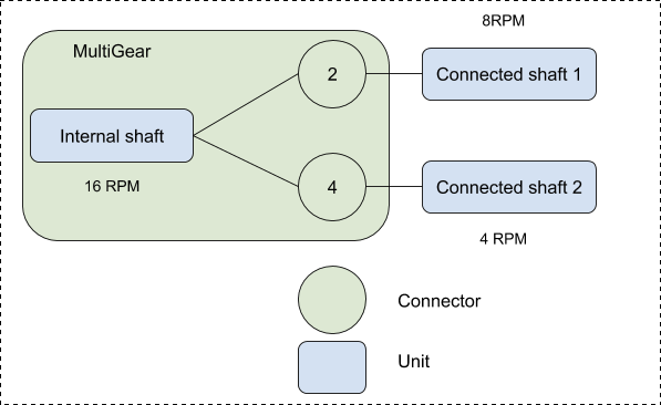
Fig. 19.6 MultiGear schematic.

// Create an internal shaft that acts as the input to the multi gear
agxDriveTrain::ShaftRef internalShaft = new agxDriveTrain::Shaft();

// Create two output shafts that will receive power from the multi gear
agxDriveTrain::ShaftRef outputShaft1 = new agxDriveTrain::Shaft();
agxDriveTrain::ShaftRef outputShaft2 = new agxDriveTrain::Shaft();

// Create a MultiGear, and add it to the power line
agxDriveTrain::MultiGearRef multiGear = new agxDriveTrain::MultiGear();

powerLine->add(internalShaft);
powerLine->add(outputShaft1);
powerLine->add(outputShaft2);
powerLine->add(multiGear)

// Set the gear ratio for each output shaft
multiGear->setGearRatio(outputShaft1, 2.0);
multiGear->setGearRatio(outputShaft2, 4.0);

// Connect the shafts to the multi gear
// This completes the power transmission paths:
// internalShaft → multiGear → outputShaft1 / outputShaft2
internalShaft->connect(multiGear);
multiGear->connect(outputShaft1);
multiGear->connect(outputShaft2);

Note

A MultiGear only supports connections on the output side.

19.7. Differential

A Differential is a Connector that distributes torque evenly over multiple output shafts. It ensures that the angular velocity of the input shaft equals the average of the velocities of the output shafts.

The differential can be locked, forcing all outputs to rotate at the same speed. Additionally, it supports a limited slip torque mode, which allows only a limited amount of torque to be transferred between outputs. This helps maintain equal output shaft velocities while still permitting slight differences when necessary.

19.7.1. Example Usage

The example below shows how to create a differential and connect it to two wheel actuators, enabling torque distribution between the left and right wheels so they can rotate at different speeds for smooth and realistic cornering behavior.

// Create an input shaft that delivers power into the differential
agxDriveTrain::ShaftRef inputShaft = new agxDriveTrain::Shaft();

// Create a differential, which splits torque between two output shafts (wheels)
// allowing them to rotate at different speeds — essential for smooth cornering
agxDriveTrain::DifferentialRef differential = new agxDriveTrain::Differential();

// Create two rotational actuators that will drive the left and right wheel hinges
agxPowerLine::RotationalActuatorRef leftWheelActuator = new agxPowerLine::RotationalActuator(left_wheel_hinge);
agxPowerLine::RotationalActuatorRef rightWheelActuator = new agxPowerLine::RotationalActuator(right_wheel_hinge);

// Add all drivetrain components to the power line
// The power line manages the dynamic interaction between these components
powerLine->add(inputShaft);
powerLine->add(differential);
powerLine->add(leftWheelActuator);
powerLine->add(rightWheelActuator);

// Connect the drivetrain components to form the complete power flow:
// inputShaft → differential → leftWheelActuator / rightWheelActuator
inputShaft->connect(differential);
differential->connect(leftWheelActuator);
differential->connect(rightWheelActuator);

19.8. Brake

The Brake, as shown in Fig. 19.7, is a mechanism that applies a counteracting torque to a rotor, gradually reducing its rotational motion until it comes to a complete stop.

A typical brake assembly consists of the caliper, brake pads, and hydraulically actuated pistons. The pistons press the brake pads firmly against the rotating disc, generating friction and slowing down the rotor. Fig. 19.7 (b) shows the operational sequence of the brake, detailing both the engagement and disengagement processes. It illustrates how the components interact as the brake is applied and released.

The fraction, denoted as \(f\), represents the position of the brake pedal relative to the motion of the brake pads during braking operations.

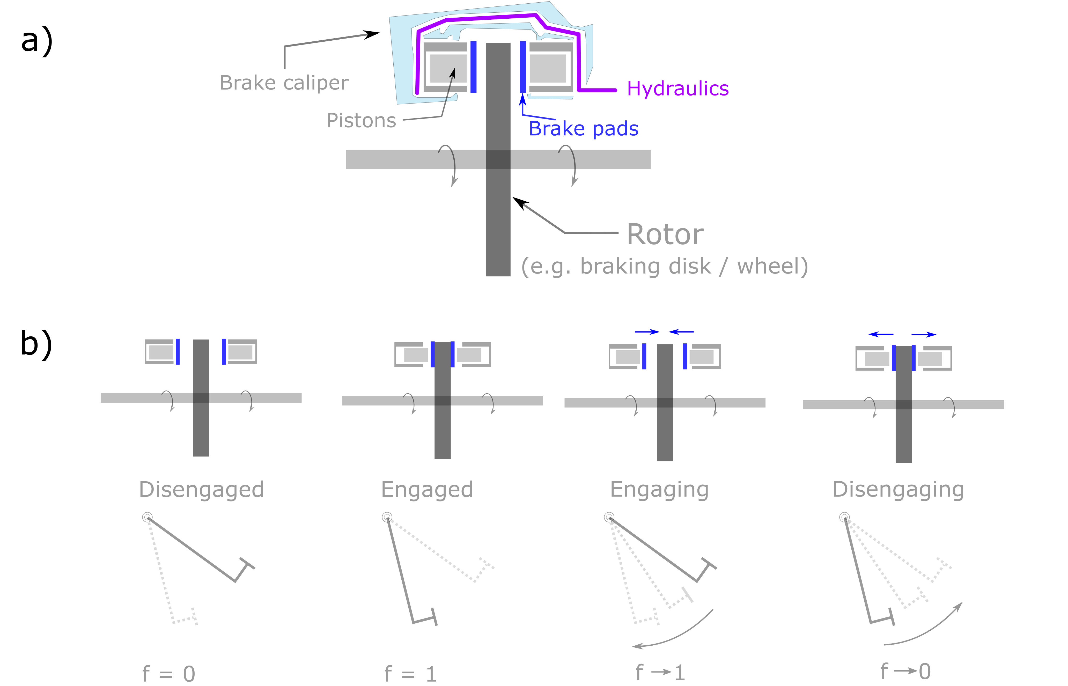
Fig. 19.7 Brake schematic. (a) Typical assembly; (b) Working mechanism.

A value of \(0\) indicates that the brake is fully disengaged – the pedal is fully released, and no braking torque is applied (free rotation). A value of \(1\) means the brake is a fully engaged – the pedal is fully pressed, and maximum braking torque transfer is applied. During the engaging and disengaging process, \(f\) varies within \([0, 1]\), simulating the varying braking force based on the pedal position.

The brake operates similarly to a DryClutch, but in reverse. While a clutch engages when the pedal is released, a brake engages when the pedal is pressed. Because of their mechanical similarity, both the Brake and DryClutch share a unified API interface, reflecting their closely related operational principles.

19.8.1. Governing equations

In AGX, the brake is modelled as a velocity (nonholonomic) constraint attached to a rotational Shaft. The constraint is expressed as

\[0 = \omega \perp \tau \in[-\tau_{C},\tau_{C}],\]

where - \(\omega\) refers to the angular speed of the shaft, - \(\tau\) is the torque transmitted through the brake pad, - \(\tau_{C}\) is the maximum torque capacity.

The perpendicularity condition (\(\perp\)) implies that either:

• \(\omega = 0\) and \(-\tau_{C} < \tau < \tau_{C}\), or

• \(\omega > 0\) and \(\tau = -\tau_{C}\), or

• \(\omega < 0\) and \(\tau = \tau_{C}\).

This constraint regulates the shaft’s rotation by controlling the magnitude of the torque applied, with two key configurable parameters: the fraction \(f\) and the torque capacity \(\tau_{C}\).

The torque capacity \(\tau_{C}\) depends on the properties of the brake pads and defines the maximum amount of transferable torque. A higher torque capacity leads to a stronger braking effect, enabling quicker deceleration as the brake pedal position increases. By adjusting the brake pedal position and torque capacity, the brake model can simulate different braking behaviors – from gradual deceleration to a more immediate stop.

When the lock (the positional, or holonomic constraint) is activated, the following constraint is enforced:

\[0 = \phi,\]

where \(\phi\) refers to the angular position of the shaft. This models a parking brake mechanism, keeping the shaft stationary with no limits on the applied torque.

19.8.2. Parameters

The physical parameters of the Brake are listed below.

Parameter	Method	Description	Default
\(f\)	setFraction	Fraction of the brake pedal position (or equivalently, the fraction of the maximum counter torque applied by the brake pads). Ranges from 0 to 1.	0
\(\tau_{C}\)	setTorqueCapacity	Maximum torque that the brake pads can transfer (N·m)	2000
autoLock	setAutoLock	Enable or disable automatic locking	True
engageTimeConstant	setEngageTimeConstant	Time required to transition the brake from disengaged to engaged. The unit matches the user-defined time step. A value of \((0, \infty]\) indicates that the brake pedal remains in its current position.	2.5
disengageTimeConstant	setDisengageTimeConstant	Time required to transition the brake from engaged to disengaged.	1.0
minRelativeSlip	setMinRelativeSlip	Threshold for checking whether the lock criterion is fulfilled (dimensionless).	1e-5
manual	setManualMode	Set brake to manual or automatic control mode (See Brake manipulation)	False
engage	setEngage	Activate (True) or deactivate (False) the braking engagement operation	False

Users can adjust these parameters to achieve desired braking performance, responsiveness, and driving characteristics.

19.8.3. Build brake

A brake can be created and configured as follows:

agxPowerLine::PowerLineRef powerLine = new agxPowerLine::PowerLine();
agxDriveTrain::BrakeRef brake = new agxDriveTrain::Brake();
brake->setTorqueCapacity(1000.0);
brake->setEngageTimeConstant(0.2);
brake->setDisengageTimeConstant(1.0);
brake->setAutoLock(true);
powerLine->add(brake);

Once built, the brake can be connected to other DriveTrain components.

19.8.4. Brake manipulation

The brake can operate in two modes: manual and automatic.

In the manual mode, the user can in great detail control the operation of the brake using the setFraction() method, see the code snippet below:

class ManualBrakeListener : public agxSDK::StepEventListener
{
  public:
    ManualBrakeListener(agxDriveTrain::Brake* brake) : m_brake(brake)
    {
    }
    void pre(const agx::TimeStamp& t)
    {
      // Disengaged
      if (t < 1.0) {
        m_brake->setFraction(0.0);
      }
      // Engaging
      else if (t <= 1.1) {
        m_brake->setFraction(10 * (t-1));
      }
      // Disengaging
      else if (t <= 3.0) {
        m_brake->setFraction((3.0-t)/(3-1.1));
      }
  private:
    agxDriveTrain::Brake* m_brake;
  }

In this example, the brake begins engaging rapidly at t=1 s and is fully engaged at t=1.1 s. It then disengages gradually, becoming fully disengaged at t=3.0 s.

In the automatic mode, the brake can be controlled using setEngage() method:

class AutoBrakeListener : public agxSDK::StepEventListener
{
  public:
    AutobrakeListener(agxDriveTrain::Brake* brake) : m_brake(brake)
    {
    }
    void pre(const agx::TimeStamp& t)
    {
      // Engaging
      if (t > 3.0 && t <= 5.0)
      {
        m_brake->setEngage(true);
        // Engage goes from 0 to 1 in 2 seconds.
        m_brake->setEngageTimeConstant(2.0);
      }
      // Disengaging
      else if (t> 7.0 && t <= 9.0)
      {
        m_brake->setEngage(false);
        // Disengage goes from 1 to 0 in 1 seconds.
        m_brake->setDisengageTimeConstant(1.0);
      }
      // Brake on-hold
      else {
        m_brake->setEngageTimeConstant(agx::Infinity );
        m_brake->setDisengageTimeConstant(agx::Infinity );
      }
  private:
    agxDriveTrain::Brake* m_brake;
  }

Comprehensive C++ and Python examples with Brake() can be found in:

• <agx_dir>/tutorials/tutorial_driveTrain_combustionEngine.cpp,

• <agx_dir>/data/python/tutorials/tutorial_driveTrain_brake.agxPy, and

• <agx_dir>/data/python/tutorials/tutorial_driveTrain_combustionEngine.agxPy.

19.9. Actuator

An Actuator is a PowerLine component that transfers motion between a powerline Unit and a standard AGX constraint such as a Hinge or Prismatic.

Since a Hinge represents rotational constraint and a Prismatic represents translational constraint, there are two specialized subclasses of the Actuator class:

• agxPowerLine::RotationalActuator – connects to rotational constraints (e.g., hinges).

• agxPowerLine::TranslationalActuator – connects to translational constraints (e.g., prismatic joints).

19.9.1. Example Usage

If a wheel body is attached to a chassis via a hinge named hinge, the wheel can be powered through the drivetrain as follows:

// Create a rotational actuator linked to the hinge constraint
agxPowerLine::RotationalActuatorRef actuator = new agxPowerLine::RotationalActuator(hinge);

// Connect an existing drivetrain (shaft) to the hinge via the RotationalActuator.
shaft->connect(actuator);

This establishes a link between the drivetrain shaft and the hinge, allowing torque and rotational motion to be transmitted through the PowerLine system.

19.10. WireWinchActuator

A winch is a rotating drum used to spool wire in or out. Its effective radius changes depending on how much wire is currently wound on the drum. To simulate a torque-driven winch, it must be connected to a rotational power source, such as a motorized Hinge or an Engines.

The agxWire::WireWinchController manages winch operation by controlling the motor and brake. It acts as a linear constraint, applying a linear force (in Newtons) along the wire to simulate real winching behavior.

Since the winch mechanism operates linearly while the power source operates rotationally, AGX uses agxPowerLine::RotationalTranslationalHolonomicConnector to convert rotational motion to linear motion.

To connect this converter to the winch, use agxPowerLine::WireWinchActuator, which bridges rotational and linear power transmission, ensuring physically consistent torque-to-tension conversion.

By combining:

• a motorized hinge (rotational input),

• a RotationalTranslationalHolonomicConnector (conversion element), and

• a WireWinchActuator (link to the winch),

AGX provides a robust framework for simulating realistic wire and rope systems that accurately transform motor torque into wire tension.

19.10.1. Example Usage

The following example demonstrates how to integrate a WireWinchActuator into a AGX PowerLine system. It shows how rotational motion from a motorized hinge is converted into linear motion to drive a winch through a RotationalTranslationalHolonomicConnector.

// PowerLine chain:
//   [Hinge]
//      ↓
//   [Shaft]
//      ↓
//   [RotationalTranslationalHolonomicConnector]
//      ↓
//   [WireWinchActuator]
//      ↓
//   [Winch]

// Assume we have a pointer to a winch object with a routed wire.
// Create a shaft that transfers rotational motion from the motorized hinge to the connector.
auto shaft = new agxDriveTrain::Shaft();
auto winch_socket = new agxPowerLine::RotationalTranslationalHolonomicConnector();

// Define the effective radius of the winch drum.
// This determines the relationship between the hinge’s rotational motion and the winch’s linear motion.
// A larger radius produces higher linear speed but lower pulling force.
winch_socket->setShaftRadius( radius );

// Connect the shaft to the winch_socket
shaft->connect( winch_socket );
shaft->setInertia( 1e-4 ); // Approximate inertia of the rotating drum

// Add the shaft to the PowerLine system.
power_line->add( shaft );

// Create a hinge aligned with the shaft’s rotational axis.
auto frame = new agx::Frame();
frame->setLocalRotate( agx::Quat( agx::Vec3::Z_AXIS(), shaft->getRotationalDimension()->getWorldDirection())  );

// Initialize the hinge constraint.
auto winch_hinge = new agx::Hinge( shaft->getRotationalDimension()->getOrReserveBody(), frame );

// Initially, keep the hinge locked and disable the motor.
// To start winching, unlock the hinge and enable the motor with a target speed.
winch_hinge->getMotor1D()->setEnable( false );
winch_hinge->getMotor1D()->setSpeed( 0 );

// Note: Lock1D is not a brake — it behaves like a spring when its target position is exceeded.
// To prevent "springback", either update the lock target position dynamically
// or replace it with a friction-based controller.
winch_hinge->getLock1D()->setEnable( true );
simulation->add( winch_hinge );

// Create an actuator that transfers linear motion from the connector to the winch.
auto winch_actuator = new agxPowerLine::WireWinchActuator( winch );

// Connect the actuator to the connector and register it in the PowerLine system.
winch_socket->connect( winch_actuator );
power_line->add( winch_actuator );

For a more complete example, see <agx_dir>/data/python/torque_driven_winch.agxPy.

19.11. Clutch (deprecated)

Note

The class Clutch has been deprecated. It is recommended to use DryClutch instead.

A clutch is a Connector with configurable efficiency and torque transfer characteristics.

The efficiency parameter ranges from 0 to 1, where:

• 0 corresponds to no torque transfer (fully disengaged), and

• 1 represents a rigid coupling (fully engaged).

The torque transfer constant define the shape of the torque transfer curve as the efficiency varies between 0 and 1. A larger constant results in a steeper torque response, meaning torque increases more rapidly as efficiency rises.