59. Appendix 5: Robot control demo
This section will describe how to control the position of a robot by driving each joint with a motor that adds forces to the joint, to keep it in the right position. Each robot joint will be controlled independently, based on a trajectory file describing the angle of each joint at each time step. A drive line together with a PID controller will then be used to add the correct torques to the joints.
Most of the scripts used in this demo are located under the folder RobotControl among the python tutorials.
59.1. PID controller demo
We start with a simple example of how to use a PID controller on a single joint arm. First we take a look at the PID controller. We use a simple example, which can be found in Figure 11.15 in Modern Robotics: Mechanics, Planning, and Control, by K. M. Lynch and F. C. Park.
59.1.1. PID controller
The PID controller is implemented as a StepEventListener and will need the joints we want to control, the file with the trajectory and the PID tuning parameters. The heart of the PID controller is the calculation of the regulator torque, \(\tau\), which mathematically can be expressed as
where \(\theta_e\) is the difference between the current angle and the reference angle and \(K_p\), \(K_d\) and \(K_i\) are the tuning parameters.
In the controller used in this demo, \(\dot{\theta_e}\) is calculated as the difference between the wanted angular velocity and the current velocity, where the velocities are approximated by dividing the change in angle from the previous step with the time step. The integral part is approximated by adding up the error, \(\theta_e\), multiplied with the time step.
For more details about the implementation of the PID controller, see pid_controller.py.
In pid_controller.py there is also a class called RobotJoint, which is used to save a hinge and the lookup table used to set the torque for that hinge. The hinges we want to control must be saved into a RobotJoint before it is sent into the PID controller.
59.1.2. Single joint simulation
To test the PID controller a single joint arm is created. It is simply a long and thin box connected to a static body with a hinge. To drive the hinge a drive line with an engine is created, connected to the hinge with a gear. The engine is mainly used since it makes it simple to control what torque is applied to the drive line. The torque is added as the only value in the engine lookup table, which is saved together with the hinge as a RobotJoint.
hinge.getMotor1D().setEnable(False)

powerLine = agxPowerLine.PowerLine()
sim.add(powerLine)

engine = agxDriveTrain.Engine()
engine.setPowerGenerator(agxPowerLine.TorqueGenerator(engine.getRotationalDimension()))
engine.setThrottle(1)
lookupTable = engine.getPowerGenerator().getPowerTimeIntegralLookupTable()
powerLine.add(engine)

actuator = agxPowerLine.RotationalActuator(hinge)
gear = agxDriveTrain.HolonomicGear()
engine.connect(gear)
gear.connect(actuator)

joint = RobotJoint(hinge, lookupTable)
The PID controller must know what angle the joint should have at what time, and in this case it reads it from a trajectory file. This file must thus first be created. As this example only has one joint, it is easy to add the angles and corresponding times into each line of a file. We let the arm move up to \(\frac{\pi}{2}\) rad in 2 seconds, rest there for a second and then move down again in 2 seconds. To get a smooth trajectory the controller gets one angle position for each time step, except when the arm should be standing still.
time = np.append(np.linspace(0, 2.0, 2000), np.linspace(3.0, 5.0, 2000))
angle = np.append(np.linspace(0, agx.PI/2, 2000), np.linspace(agx.PI/2, 0, 2000))

fileName = "single_joint_trajectory.txt"
file = open(fileName, "w")
for i in range(0, len(time)):
    file.write("{0:.4f} {1:.6f}\n".format(time[i], angle[i]))
file.close()
Having created the trajectory file it is possible to create the PID controller and add it to the simulation.
Kp = 300.0
Kd = 50.0
Ki = 50.0
controller = PidController([joint], Kp, Kd, Ki, fileName)
sim.add(controller)
The PID tuning parameters of the controller are only a suggestion, but running the example for the single joint arm with those values, should give the results seen in the figure below.
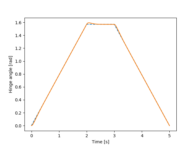
Fig. 59.1 Hinge angle for each time step. Dashed line is the reference.
For more details see tutorial_pid_controller.agxPy.
59.2. Generic robot demo
In this tutorial it is demonstrated how to control a robot with six degrees of freedom. The robot used is the GenericRobot. See figure below.
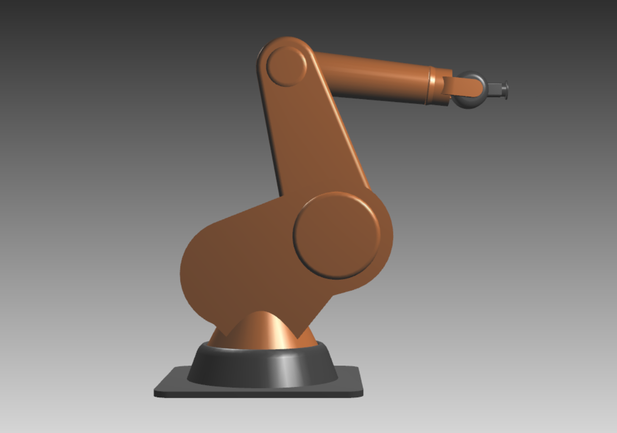
Fig. 59.2 The robot called generic robot.
59.2.1. Generating a trajectory
To control the robot and move it into some wanted position or pattern it must first be known how each of the joints in the robot should move. In this case the joints are controlled independently and a file is created with angle positions for each joint at each time step.
Normally the angles of the joints are not known, but what is known is the position of where the end effector should be. This is a problem that can be solved in more than one way, but here only one, simple, solution is demonstrated. The approach is to drag the end effector into the wanted position, and collect the joint angles during the motion. This is done by creating a kinematic body and connecting it to the robot head. The kinematic body is then moved in straight lines to the wanted positions. One must be careful not to move this body into a position outside the reach of the robot. The velocity of this body is constant between the positions, but for better results it is possible to make it slow down as it comes closer to its destination.
In the example in tutorial_robot_trajectory.agxPy the kinematic body moves in a square in a horizontal plane and saves that angle data into a file named trajectory_square.txt.
59.2.2. Controlling a robot
Having the trajectory of the robot, it is possible to try to move the robot in the same pattern using a PID controller and something that drives the joints. Just as for the single joint example an engine in a drive train is connected to the hinge with a gear and in this case we set the engine inertia and gear ratio to a given value. Then a RobotJoint must be created for each joint using the correct hinges and lookup tables.
# Save all the hinges of the robot in a list
hinges = [robot.hinges["bottom"], robot.hinges["bottomMiddle"], robot.hinges["middleTop"],
          robot.hinges["topHead"], robot.hinges["head"], robot.hinges["headPlate"]]

# List of values for motor inertia and gear ratio.
motorInertia = [0.27, 0.046, 0.036, 0.15, 0.15, 0.18]
gearRatio = [125.0, 171.0, 143.0, 60.0, 67.0, 50.0]

powerLine = agxPowerLine.PowerLine()
sim.add(powerLine)

joints = []
for i in range(0, len(hinges)):
    hinges[i].getMotor1D().setEnable(False)
    engine = agxDriveTrain.Engine()
    engine.setPowerGenerator(agxPowerLine.TorqueGenerator(engine.getRotationalDimension()))
    lookupTable = engine.getPowerGenerator().getPowerTimeIntegralLookupTable()
    engine.setThrottle(1.0)
    engine.setInertia(motorInertia[i])
    powerLine.add(engine)

    actuator = agxPowerLine.RotationalActuator(hinges[i])
    gear = agxDriveTrain.HolonomicGear()
    gear.setGearRatio(gearRatio[i])

    engine.connect(gear)
    gear.connect(actuator)

    joints.append(RobotJoint(hinges[i], lookupTable))
A PID controller can then be created. Note that only one controller is needed. The joints should all be put in a list, that is sent into the controller. The tuning parameters can either be set to the same value for all joints, by just sending in one value, or to different values for each joint. If one wants different parameter values for each joint, the parameters are put in a list instead. The order has to be the same as for the joints, i.e. the first value is for the first joint and so on.
sim.add(PidController(joints, 900, 200, 600, "trajectory_square.txt"))
Running the tutorial with the square example with the above controller should give the result seen in the figure below.
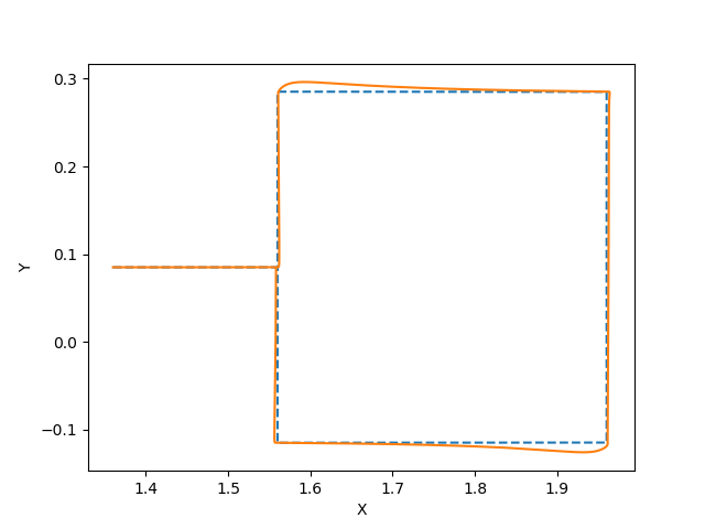
Fig. 59.3 Robot tool position in the x-y-plane. The values are in meters and the dashed line is the reference. The robot follows the straight line to the square, then moves clockwise around the square path.
For more details see tutorial_robot_control.agxPy.