12. Creating objects

12.1. RigidBody

An agx::RigidBody is an entity in 3D space with physical properties such as mass and inertia tensor and dynamic properties such as position, orientation and velocity. A rigid body is created as follows:

agx::RigidBodyRef body = new agx::RigidBody();
simulation->add( body ); // Add body to the simulation

There are three motion control schemes for a RigidBody:

Table 12.1 Motion control modes for a rigid body

DYNAMICS	Affected by forces, position/velocity is integrated by the DynamicsSystem.
STATIC	Not affected by forces, considered to have infinite mass, will not be affected by the integrator.
KINEMATICS	Controlled by the user. By supplying a target transformation and a delta time, a linear and an angular velocity are calculated. This velocity will be used by DynamicsSystem to interpolate the position/orientation of the kinematic RigidBody. The angular velocity is considered to be constant during the interpolation.

The type of motion control is set with the method:

RigidBody::setMotionControl(RigidBody::MotionControl);

12.1.1. Velocities

The angular and linear velocity of a rigid body is always understood as the velocity of the center of mass. Velocities of a rigid body are expressed in the world coordinate system.

agx::Vec3 worldVelocity(0,1,0);

// Specify the linear velocity in world coordinates for a rigid body
body->setVelocity( worldVelocity );

// Specify angular velocity for a body in LOCAL coordinate system
agx::Vec3 localAngular(0,0,1);

// Convert from local to world coordinate system
agx::Vec3 worldAngular = body->getFrame()->transformVectorToWorld( localAngular);

// Set the angular velocity in World coordinates
body->setAngularVelocity( worldAngular );

12.2. Effective Mass

When for example simulating a ship in water, the effective mass can be substantially larger than the actual weight of the ship. This is due to the water that is added by hydrodynamic effects. The mass varies depending on depth of water and is also different in different directions. The class agx::MassProperties has the capability of handling this added mass through the methods:

void setMassCoefficients( const Vec3& coefficients );
void setInertiaTensorCoefficients(const Vec3& coefficients);

This also means that AGX can handle objects that have different masses along each axis, so called non-symmetric mass matrices.

12.3. Modeling coordinates/Center of Mass coordinates

Center of mass is the point in the world coordinate system where the collected mass of a rigid body is located in space. This point can either automatically be calculated from the geometries/shapes that are associated to the rigid body, or it can also be explicitly specified to any point in space.

Since the center of mass moves when geometries are added (if RigidBody::getMassProperties()::getAutoGenerate()==true), it is not a practical reference when building a simulation. For example, if a constraint is attached to a body relative to the body center of mass, adding another geometry and thereby moving the center of mass would change to attachment point for the constraint. This is usually not the expected/wanted behavior.

Therefore AGX provides two coordinate frames, the model frame and the center of mass(CM) frame.

Fig. 12.1: shows one box with the model origin (axes) and the center of mass (yellow sphere) at the same positions. Fig. 12.2: illustrates the situation after another box geometry is added to the body, and thus the center of mass (yellow sphere) is shifted along the y-axis. The model origin (axes) is still at the same position.

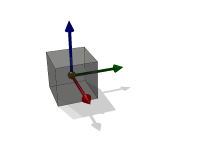
Fig. 12.1 Model and Center of mass at the same position.

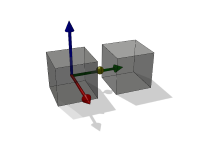
Fig. 12.2 Center of mass translated due to added geometry.

Note

AGX only supports relative translation of the center-of-mass-frame with regard to the model frame, but not relative rotation.

The translation, rotation and velocity of the center of mass for a rigid body can be accessed via the methods:

agx::RigidBodyRef body = new agx::RigidBody;

// Get position of Center of Mass in world coordinate system
Vec3 pos = body->getCmPosition();

// Get orientation of Center of Mass in world coordinate system
Quat rot = body->getCmRotation();

// Get rotation and translation of Center of Mass in world
// coordinate system
AffineMatrix4x4 m = body->getCmTransform();

// Or the complete frame at one call
Frame *cmFrame = body->getCmFrame();

// Translation relative to model coordinate system
Vec3 pos = body->getCmFrame()->getLocalTranslate();

// In most situation, it is the model coordinate system that is interesting. This can be accessed using the calls:
// Get position of Rigid Body in world coordinate system
Vec3 pos = body->getPosition();

// Get orientation of Rigid Body in world coordinate system
Quat rot = body->getRotation();

// Get rotation and translation of Rigid Body in world coordinate system
AffineMatrix4x4 m = body->getTransform();

// Or the complete frame at one call
Frame *cmFrame = body->getFrame();

// Get linear velocity of body
Vec3 v = body->getVelocity()

/**
\return the local offset of the center of mass position to the model origin (in model frame coordinates).
*/
agx::Vec3 getCmLocalTranslate() const;

/**
Sets the local offset of the center of mass position to the model origin (in model frame coordinates).
\param translate The new offset.
*/
void setCmLocalTranslate(const agx::Vec3& translate);

12.4. Kinematic rigid body

By specifying that a rigid body should be kinematic, we are telling the DynamicsSystem to stop simulating the dynamics of the body. This means that it will get an infinite mass, will not be affected by forces etc.

rigidbody->setMotionControl( agx::RigidBody::KINEMATICS );

It is also possible to interpolate the position/orientation based on a target transformation specified by the user. The body can then be specified to move from the current transform to a new during a specified time step with the call to:

agx::RigidBody::moveTo(AffineMatrix4x4& transform, agx::Real dt);

The above method will make a body move in a velocity calculated from its current transformation frame, to the specified during a time interval of dt.

When the interval dt is reached (current time + dt) the body will continue to move according to its velocity until next call to moveTo().

If you explicitly set a linear/angular velocity on a body, and specify it to be KINEMATICS, then that velocity will be used for integrating the transformation (position and orientation).

12.5. Geometry

A Geometry can be assigned to a rigid body to give it a geometrical representation. The geometry is also the entity that can intersect other geometries and create contacts. A Geometry contains one or more shapes. A Shape is specialized by Box, Sphere, Capsule etc. see table 12.4 for a complete list of available shapes.

12.5.1. Enable/disable

A Geometry can be enabled/disabled. A disabled geometry will not be able to collide with any other geometries. This is true for all the shapes in the geometry. A disabled geometry will not contribute to the mass properties of a rigid body.

void Geometry::setEnable( bool enable );
bool Geometry::getEnable() const;
bool Geometry::isEnabled() const;

Calling geometry->setEnable(false) will effectively remove the geometry from the mass calculation and collision detection.

12.5.2. Sensors

A geometry can be specified to be a sensor. This means that the collision system will generate contact information, such as contact points, normals and penetration, but no physical contact (contact constraint) will be created, hence the solver will not see this contact. A sensor can therefore penetrate any other geometry as a “ghost”. This can be useful for realizing certain functionality such as proxy tests, vision etc. A geometry is specified to be a sensor through the call:

agxCollide::GeometryRef geometry = new agxCollide::Geometry;
geometry->setSensor( true ); // Tell the geometry to become a Sensor

A sensor geometry will not add any physical properties such as mass, center of mass, or inertia tensor to the body it is part of. Calling setSensor(true) will effectively remove the geometry from the mass calculation.

In some cases it is enough to know that a sensor overlapped with some other geometry, without any need for the contact point data. Performance can be improved by not computing that data and instead letting the collider do an early out as soon as possible when an overlap has been detected. Contact data generation is disabled for a sensor geometry by passing false as the second argument to setSensor:

geometry->setSensor(true, false);

Disabling contact generation on a geometry that isn’t a sensor has no effect, contact points will always be generated for geometries that aren’t sensors.

Support for collider early out is added on a shape-type-pair basis and not all pairs are handled yet. Currently supported are:

• box-trimesh

• cylinder-trimesh

• sphere-trimesh

12.6. Enabling/disabling Contacts

There are several different alternatives to control whether pairwise contacts should occur or not.

• Disable all collisions for a geometry: Geometry::setEnableCollisions(false)

• Enable/disable pair of geometries

• Geometry groups

• User supplied contact listeners

It should be noted that there is not direct priority between these different possibilities, but rather, if any of them disables the contact (even if others enable it), the contact generation will be treated as disabled.

12.6.1. Disable collisions for a geometry

To explicitly disable all collision generation for a geometry:

// Disable all contact generation for the geometry:
geometry1->setEnableCollisions( false );

12.6.2. Enable/disable pair

To disable/enable contacts for a specific geometry pair one can call the method Geometry::setEnableCollisions( Geometry*, bool )

// Disable contact generation between geometry1 and geometry2
geometry1->setEnableCollisions( geometry2, false );

// Enable contact generation between geometry1 and geometry2
geometry1->setEnableCollisions( geometry2, true );

No matter if any of the two geometries are removed and later added to simulations, the information about setEnableCollisions() will still be available.

12.6.3. GroupID

The class Geometry has a groupID attribute. This attribute can be set and read using the following methods:

void agxCollide::Geometry::addGroup( unsigned );
bool agxCollide::Geometry::hasGroup( unsigned ) const;
bool agxCollide::Geometry::removeGroup( unsigned );

With the method addGroup() one can assign a geometry to a specified group of geometries.

Together with the following method in agxCollide::Space:

void agxCollide::Space::setEnablePair(unsigned id1,
                                                        unsigned id2,
                                                        bool enable)

This functionality can be used to disable collisions between groups of geometries. To disable collisions between geometries of the same group:

space->setEnablePair( id1, id1, false );

After the above call, geometries belonging to id1 cannot collide with each other. t is worth to notice that the group ids are stored in a vector, so searching and comparing has a time complexity of O(n). So before adding a large number of group ids to a geometry, make sure there isn’t another alternative. This is because the geometry groups will be compared to each other during the collision detection process.

12.6.4. Named collision groups

New in 2.3.0.0 is that there is also named collision groups. This has the same functionality as GroupID, but it is defined using a string instead.

void agxCollide::Geometry::addGroup( const agx::Name& );
bool agxCollide::Geometry::hasGroup(const agx::Name& ) const;
bool agxCollide::Geometry::removeGroup(const agx::Name& );

This functionality can be used to disable collisions between groups of geometries. To disable collisions between geometries of the same group:

space->setEnablePair( name1, name1, false );

After the above call, geometries belonging to name1 cannot collide with each other.

12.6.5. User supplied contact listener

A ContactEventListener (see 11.4.3) can be registered to listen to specific collision events, between specified geometries, geometries with specific properties etc. By implementing a collision event listener that for a given pair of geometries return REMOVE_CONTACT or KEEP_CONTACT immediately in the impact() method, one can achieve the same result as the previous two alternatives, namely, no contact is transferred to the contact solver. This is a very general way of specifying for which pairs contacts should be generated.

class MyContactListener : public agxSDK::ContactEventListener
{
public:
  MyContactListener()
  {
    // Only activate upon impact event
    setMask(agxSDK::ContactEventListener::IMPACT);
  }

  bool impact(const agx::TimeStamp& t, agxCollide::GeometryContact *cd) {

    RigidBody* rb1 = cd->geomA->getBody();
    RigidBody* rb2 = cd->geomB->getBody();

    // If both geometries have a body, and the mass of the first is over 10
    // then remove the contact
    if (rb1 && rb2 && rb1->getMassProperties()->getMass() > 10 )
      return REMOVE_CONTACT; // remove contact.

    return KEEP_CONTACT; // keep the contact
  }
};

Which geometries should trigger the ContactEventListener can be specified using an ExecuteFilter. This filter can also be user specified. By deriving from the class agxCollide::ExecuteFilter and implementing two methods, any user supplied functionality can be implemented for filtering out contacts:

class MyFilter : public agxCollide::ExecuteFilter
{
public:

  MyFilter() {}

  /**
  Called when narrow phase tests have determined overlap (when we have
  detailed intersection between the actual geometries).
  Return true if GeometryContact matches this filter:

  if both geometries have a body.
  */
  virtual  bool operator==(const agxCollide::GeometryContact& cd) const
  {
    bool f =
      (cd.geomA->getBody() && cd.geomB->getBody());
    return f;
  }

  /**
  Called when broad phase tests have determined overlap between the two
  bounding volumes.
  */
  virtual  bool operator==(const GeometryPair& geometryPair) const
  {
    bool f =
      (cd.geomA->getBody() && cd.geomB->getBody());
    return f;
  }
};

12.6.6. Surface velocity

A geometry can be given a surface velocity. It is specified in the local coordinate system of the geometry and can be used for simulating the surface of a conveyor belt. In its general form, it is independent of the contact point position relative to the geometry. If more control over that behavior is desired, it is possible to create a class inheriting from agxCollide::Geometry, and to override the method

agx::Vec3f Geometry::calculateSurfaceVelocity( const agxCollide::LocalContactPoint& point ) const.

One such class is agx::SurfaceVelocityConveyorBelt, which is described in Section 24.

12.7. Primitives for collision detection (Shapes)

AGX allows for different shapes for geometric representation. Simpler shapes such as Box, Sphere or Cylinder allow for exact representation of simple geometry, as well as fast compute times.

Mesh types such as Trimesh, Convex or HeightField allow for more complex geometry, at the cost of higher compute times.

12.7.1. Box

A box is defined by three half extents with its center of mass at origin.

Box::Box( const agx::Vec3& halfExtents )

12.7.2. Sphere

A sphere is defined by its radius and is created with its center of mass at origin.

Sphere::Sphere( const agx::Real& radius )

12.7.3. Capsule

A capsule is a cylinder, capped with two spheres at the end. It is defined by its height and its radius. The capsule will be created with its height along the y-axis and its center of mass at origin.

Capsule::Capsule( agx::Real radius, agx::Real height )

12.7.4. Cylinder

Cylinder::Cylinder( const agx::Real& radius, const agx::Real& height )

12.7.5. HollowCylinder

A hollow cylinder is similar to a cylinder but with a circular hole.

HollowCylinder::HollowCylinder( agx::Real innerRadius, agx::Real height, agx:Real thickness )

This shape is suitable for modeling peg-in-a-hole kind of scenarios in combination with other cylinders, hollowcylinders or different kinds of cones.

Note

A current limitation is that the hollow cylinder does not have full collision support against all other shape types. Until full support is available according to table 12.4, a fallback is used which treats the HollowCylinder as a Cylinder.

To give an example, the pair HollowCylinder - Sphere does not have full support and hence the sphere can not be sent through the hollow part of the cylinder due to the hollow cylinder being treated as a cylinder shape.

12.7.6. Line

A line is defined by two points, begin and end points:

Line::Line( const agx::Vec3& start, const agx::Vec3& end )

12.7.7. Plane

A plane can be defined in a number of different ways: either by a point and a normal, or the four plane coefficients:

Plane::Plane( agx::Real const a, agx::Real const b,
                  agx::Real const c, agx::Real d )
Plane::Plane( const agx::Vec3& normal , agx::Real d )
Plane::Plane( const agx::Vec3& normal, const agx::Vec3& point )
Plane::Plane( const agx::Vec4& plane)
Plane::Plane( const agx::Vec3& p1, const agx::Vec3& p2,
              const agx::Vec3& p3)

12.7.8. Cone / HollowCone

Cone::Cone( agx::Real topRadius, agx::Real bottomRadius, agx::Real height )

HollowCone::HollowCone( agx::Real topRadius, agx::Real bottomRadius, agx::Real height, agx::Real thickness )

A Cone and a HollowCone are very similar. The main difference is that the hollow cone has a conical hole. Both cone types support a non-zero topRadius which creates a truncated cone where the top part is cut off.

The cones are defined alony the Y-axis and the bottom disc is positioned at y=0 and the top point (or top disc in case of truncation) is placed at y=height.

Note

HollowCone and Cone does not currently support all other shapes. Until each collider is implemented to take into account the actual cone shape, a fallback treating them as a Convex will be used. See table 12.4.

12.7.9. Triangle mesh

12.7.9.1. Triangle mesh construction (general case)

The triangle mesh shape in AGX supports general concave triangle meshes. The internal storage of triangle meshes in AGX is based on vertices (array of 3D points) and indices (indexes into the array of vertices), where three concurrent indices define a triangle each (a triangle list). Trimeshes share a common base class called agxCollide::Mesh with another mesh-based collision shape called agxCollide::HeightField.

A trimesh can be created using code or by reading from a support mesh file format (see Mesh reader). Below is an example of how a trimesh can be created from code or from a file

agx::Vec3Vector vertices;
agx::UIntVector indices;

// Add vertices
vertices.push_back( agx::Vec3( -0.4, -0.4, 0.0 ) );
// ...

// Add indices
indices.push_back( 1 ); // starting first triangle
indices.push_back( 0 );
indices.push_back( 2 ); // finished first triangle
indices.push_back( 0 ); // starting second triangle, reusing one vertex
// ...

// Create the collision shape based on the vertices and indices
agxCollide::TrimeshRef triangleMesh = new agxCollide::Trimesh( &vertices,
&indices, "handmade pyramid" );

And from a file:

// Create the trimesh shape from a WaveFront OBJ file:
agxCollide::TrimeshRef trimeshShape =
  agxUtil::TrimeshReaderWriter::createTrimesh(
    "torusRoundForCollision.obj");

The data will be copied by the trimesh constructor.

Furthermore, the triangles are expected to be given in counterclockwise order (counterclockwise winding/orientation). This is important since the order of the vertices defines which face of the triangle will point outwards and which inwards. This orientation is used within calculation of mass properties and collision detection. If the data is given in clockwise winding, this can be indicated by setting the according flag in agxCollide::Trimesh::TrimeshOptionsFlags. Mixed winding should be avoided since it will lead to unexpected behavior. The flag agxCollide::Trimesh::RECALCULATE_NORMALS_GIVEN_FIRST_TRIANGLE can be used to adapt the winding to the first triangle, given that the mesh is watertight otherwise.

Internally, the triangle data will be stored in counterclockwise winding.

For good collision detection results, each trimesh should be a watertight (a geometrical manifold). Non-manifold trimeshes can be used, but the results may vary in quality. Non-manifold trimeshes may furthermore result in an invalid mass and inertia when used in dynamic rigid bodies for which mass properties are calculated automatically.

12.7.9.2. Triangle meshes as terrain

Trimeshes can also be used to model terrains. Here, they do not have to be closed on all sides, but may have an open direction. This direction is assumed to be upward in z direction in the trimesh’s local coordinate system. The corresponding normal (0, 0, 1) is used as a tunneling safeguard, and the trimesh’s bounding box is enlarged in opposite direction of this normal by a value called the terrain’s “bottom margin”.

It is recommended to avoid collisions at terrain borders unless they are met by a corresponding neighboring terrain, since this might give suboptimal results. The trimesh class will give out warnings during construction if a terrain does not have a rectangular shape (in the trimesh’s local x and y coordinates), or contain holes. The usage as terrain should be indicated in the optionsMask.

One example for a terrain with a bottom margin of 5.0 below the mesh’s deepest point in Z:

agx::Vec3Vector vertices;
agx::UIntVector indices;

// Add vertices
vertices.push_back( agx::Vec3( -0.4, -0.4, 0.0 ) );
...
// Add indices
indices.push_back( 1 ); // starting first triangle

uint32_t optionsMask = agxCollide::Trimesh::TERRAIN;
...
TrimeshRef terrain = new Trimesh( &vertices, &indices, "handmade terrain", optionsMask, 5.0 );

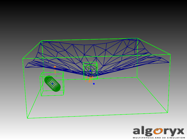
Fig. 12.3 Terrain/trimesh intersecting a box, and a capsule which is prevented from tunneling. Note the enlarged bounding box in opposite direction of the terrain normal.

Using a height-field for collision detection as a terrain has the advantage of being able to modify the terrain during run-time. Trimeshes as terrains, on the other hand, can be modeled with fewer triangles by adapting the level of detail to the local change in terrain height, so that large plain parts can be covered by few large triangles.

12.7.9.3. Triangle meshes modeling

As mentioned above, special attention should be paid when using triangle meshes as collision primitives.

It is important that the models are adapted for the special needs arising from physics simulation, and thus are either manifolds or used as terrain.

Potential problems (which should be fixed externally before using the trimesh) are:

• Unmerged identical vertices

• Holes

• Wrong/inconsistent winding

• Triangles with zero area

• Unreferenced vertices

• Self-intersection.

Trimeshes used in collision detection create potentially very many contact points. The use of contact reduction is therefore recommended.

12.7.9.4. Mesh reduction

The time for computing geometry contacts when using a triangle mesh model can be related to the complexity of the triangle mesh. I.e. the number of triangles.

agxUtil::reduceMesh is a function that can reduce the complexity of a triangle mesh by algorithmically reduce the number of edges in a process called collapsing. The goal of the mesh reduction is to reduce the number of triangles but at the same time keep the overall shape of the mesh.

The function operates on arrays of vertices and indices to be as general as possible. Below is a code snippet that demonstrates the functionality of the mesh reduction utility. The arguments are the set of vertices and indices that should be reduced, the target reduction (in percent, 1==no reduction, 0.5==50% reduction) and an aggressiveness (>0). The higher value, the more aggressive the algorithm will be, and the longer time it will take.

agxIO::MeshReaderRef reader = new agxIO::MeshReader();
reader->readFile("data/models/bunny.obj");


agx::Vec3Vector out_vertices;
agx::UInt32Vector out_indices;

double target_reduction = 0.5; // % triangles that should be left in the model after reduction
double aggressiveness = 7.0;    // A value that indicates how aggressive the reduction should be
agxUtil::reduceMesh(reader->getVertices(), reader->getIndices(),
                    out_vertices, out_indices,
                    target_reduction,
                    aggressiveness);

// Create a Trimesh with the reduced data
agxCollide::TrimeshRef mesh = new agxCollide::Trimesh(&out_vertices, &out_indices,
                                                      "Mesh",
                                                      agxCollide::Trimesh::REMOVE_DUPLICATE_VERTICES);

12.7.9.5. Triangle mesh traversal

If a trimesh is modeled in the above recommended way and thus has a half edge structure, it can be traversed via this neighborhood graph: each triangle consists of three half edges, where each half edge has a neighboring half edge in a bordering triangle, and where one half edge’s starting vertex is the other one’s ending vertex.

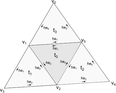
Fig. 12.4 A trimesh consisting of 4 triangles and 6 vertices. The half edge structure is shown.

This data is stored as arrays of vertices, triangle half edges and half edge neighbors in the Trimesh class and can be used directly.

Some helper classes make traversal of triangles easier, though. The neighborhood structure can be traversed by using the helper class agxCollide::Mesh::Triangle.

// Create the trimesh shape from a WaveFront OBJ file:
agxCollide::TrimeshRef trimesh =
      agxUtil::TrimeshReaderWriter::createTrimesh( "pin.obj" );
// Get first triangle in trimesh
agxCollide::Mesh::Triangle triangle = trimesh->getTriangle(0);
if (triangle.isValid()) // Important to check validity before use
      triangle = triangle.getHalfEdgePartner(0); // Get neighbor to first edge

Circling around a vertex can be done more comfortably using the helper class agxCollide::Mesh::VertexEdgeCirculator.

// Create the trimesh shape from a WaveFront OBJ file:
agxCollide::TrimeshRef trimesh =
      agxUtil::TrimeshReaderWriter::createTrimesh( "pin.obj" );
// Get a circulator around the first vertex in the first triangle.
agxCollide::Mesh::VertexEdgeCirculator circulator =
      trimesh->createVertexEdgeCirculator( 0, 0 );
// The circulator might be invalid if created from invalid parameters.
if (circulator.isValid()) {
  // Has the circulator done a whole turn around the vertex?
  while (!circulator.atEnd()) {
    // Set it to next position. The VertexEdgeIterator will even manage
    // holes in the neighborhood structure by jumping over all holes.
    circulator++;
    if (circulator.hasJustJumpedOverHole())//Have holes been passed?
      std::cout << "Vertex circulator jumped over hole\n";
  }
}

More elaborate examples can be found in tutorial_trimesh.cpp.

12.7.10. Convex

Convex is a geometry that describes a convex shape built up from a point cloud. The properties of a convex is among the following: none of the surface normals of a convex will ever cross each other, any point on a 2D projection of a convex will only be covered twice, once from the surface facing away the projection plane and once from the surface facing the projection plane.

A convex mesh can be created from a number of different sources.

1. From a triangle mesh that is known to define a convex mesh.

2. From a set of 3d points.

3. From 3d mesh files.

4. Using convex decomposition of triangle meshes.

If you have mesh data (vertices and indices) that you _know_ are convex, you can use the constructor to create a convex mesh:

agx::Vec3Vector vertices;
agx::UIntVector indices;
// We know this data to represent a convex mesh:
ConvexRef convex = new Convex(&vertices, &indices);

If you have a set of 3d points you can use the utility function in the agxUtil::ConvexReaderWriter namespace:

#include <agxUtil/ConvexReaderWriter/ConvexReaderWriter>
agx::Vec3Vector vertices;

for(size_t i=0; i < 30; i++)
{
  auto v = agx::Vec3::random( agx::Vec3(0, 0, 0), agx::Vec3(1, 1, 1) );
  vertices.push_back(v);
}

// Create the collision shape
agxCollide::ConvexRef convexMesh = agxUtil::ConvexReaderWriter::createConvex(vertices);

If you have a 3d mesh defined in a file:

#include <agxUtil/ConvexReaderWriter/ConvexReaderWriter>

// Create the collision shape
agxCollide::ConvexRef convexMesh = agxUtil::ConvexReaderWriter::createConvex("models/bunny.obj");

12.7.10.1. Convex decomposition

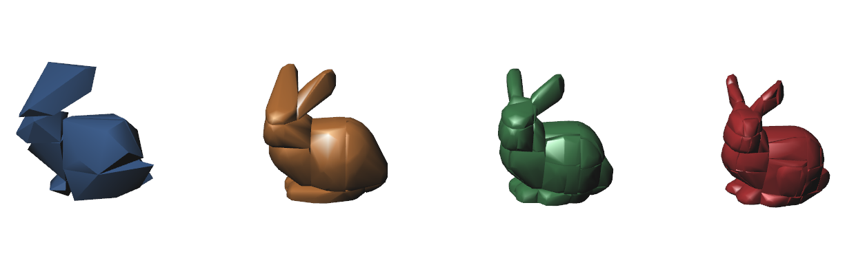
Fig. 12.5 A triangle mesh object decomposed into convex meshes with varying resolution.

The limitation of convex in that it can only describe a small subset of geometries (convex) can be overcome by taking a general (concave) triangle mesh and decompose it into convex meshes. The result will not be an exact representation of the original triangle mesh, but in many cases it will be good enough for use in simulations. AGX supports convex decomposition through the class agxCollide::ConvexFactory where you have full control over the parameterization of the algorithm.

#include <agxCollide/ConvexFactory.h>

// Create a ConvexFactory
agxCollide::ConvexFactoryRef factory = new agxCollide::ConvexFactory;

// Create a mesh reader for various mesh file formats.
agxIO::MeshReaderRef reader = new agxIO::MeshReader;
if (!reader->readFile( "mesh.obj"))
  error();

// Create a parameter object so we can fine tune the decomposition algorithm:
agxCollide::ConvexFactory::VHACDParametersRef parameters = new agxCollide::ConvexFactory::VHACDParameters();
parameters->resolution = 20;
parameters->alpha = 0.001;
parameters->beta = 0.01;
parameters->concavity = 0.01;
parameters->maxNumVerticesPerCH = 64

// Try to parse the data read from the reader and create convex shapes
size_t numConvexShapes = factory->build(reader, parameters);
if (numConvexShapes == 0)
  error();

// Get the vector of the created shapes
agxCollide::ConvexShapeVector& shapes = factory->getConvexShapes();

// Now insert shapes into one or more geometries.

An alternative is to use simpler utility function agxUtil::ConvexReaderWriter::createConvexDecomposition:

#include <agxUtil/ConvexReaderWriter/ConvexReaderWriter.h>

size_t resolution = 20;
agxCollide::ConvexShapeVector shapes
agxUtil::ConvexReaderWriter::createConvexDecomposition("mesh.obj", result, resolution);

// Now insert shapes into one or more geometries.

Below are the available parameters to the convex decomposition algorithm.

Table 12.2 Specifications of parameters to the convex decomposition algorithm

Parameter	Description	Range	Default value
resolution	maximum number of voxels generated during the voxelization stage. This will be recalculated as resolution ^3 before it reaches VHACD	[2, 400]	50
concavity	maximum concavity.	[0.0, 1.0]	0.0025
planeDownsampling	Controls the granularity of the search for the best clipping plane.	[1, 16]	4
convexhullDownsampling	Controls the precision of the convex-hull generation process during the clipping plane selection stage.	[1, 16]	4
alpha	Controls the bias toward clipping along symmetry planes.	[0.0, 1.0]	0.05
beta	Controls the bias toward clipping along revolution axes.	[0.0, 1.0]	0.05
pca	Enable/disable normalizing the mesh before applying the convex decomposition.	[false, true]	0
mode	0: voxel-based approximate convex decomposition, 1: tetrahedron-based approximate convex decomposition.	0/1	0
maxNumVerticesPerConvex	Controls the maximum number of triangles per convex hull.	[0, 1024]	64
minVolumePerConvex	Controls the adaptive sampling of the generated convex hulls.	[0.0, 0.01]	0.0001
maxConvexHulls	Maximum number of convex hulls.	[1, 1024]	1024

12.7.11. Oriented bounding volumes

Oriented Bounding Volumes (OBV) (box, cylinder, capsule) can be computed based on a set of vertices. An optimal OBV should tightly enclose the vertices to best represent the more complex shape.

Below is a code snippet that will create an oriented Box shape that will fit the given vertices. The size and the transformation are stored in the supplied arguments to agxUtil::computeOrientedBox. The transformation will contain the translation and rotation of the box relative to the coordinate system of the vertices (mesh).

// Get the vertices from an existing mesh shape
const agx::Vec3Vector& vertices = mesh->getMeshData().getVertices();

// Here is where we will store the local transformation of the oriented box relative to the Mesh
agx::AffineMatrix4x4 transform;

// Here is where we will store the size of the computed oriented box
auto halfExtents = agx::Vec3();

// Compute the size and rotation of the oriented box given the vertices
agxVerify(agxUtil::computeOrientedBox(vertices, halfExtents, transform));

// Create a box primitive based on the computed size
auto box = new agxCollide::Box(halfExtents);

// Create a Geometry including the transform that will rotate/translate the oriented bounding box relative to the mesh
auto boxGeometry = new agxCollide::Geometry(box, transform);

Alternatively an oriented Cylinder or Capsule can be created using agxUtil::computeOrientedCylinder and agxUtil::computeOrientedCapsule There is an option on how the shape should be oriented using the enum agxUtil::ShapeOrientation::Orientation. Default is agxUtil::ShapeOrientation::MINIMIZE_VOLUME which will automatically choose the principal axis of the computed shape that results in the smallest volume.

Below is code that will create an oriented cylinder based on a set of vertices.

// Get the vertices from an existing mesh shape
const agx::Vec3Vector& vertices = mesh->getMeshData()->getVertices();

// Here is where we will store the local transformation of the oriented box relative to the Mesh
agx::AffineMatrix4x4 transform;

// Here is where we will store the radius and height of the computed cylinder
auto radiusHeight = agx::Vec2();

auto orientation = agxUtil::ShapeOrientation::MINIMIZE_VOLUME; // Default

// Compute the size and rotation of the oriented box given the vertices
agxVerify(agxUtil::computeOrientedCylinder(vertices, radiusHeight, transform, orientation));

// Create a cylinder primitive based on the computed size
auto cylinder = new agxCollide::Cylinder(radiusHeight[0], radiusHeight[1]);

// Create a Geometry including the transform that will rotate/translate the oriented bounding cylinder relative to the mesh
auto boxGeometry = new agxCollide::Geometry(cylinder, transform);

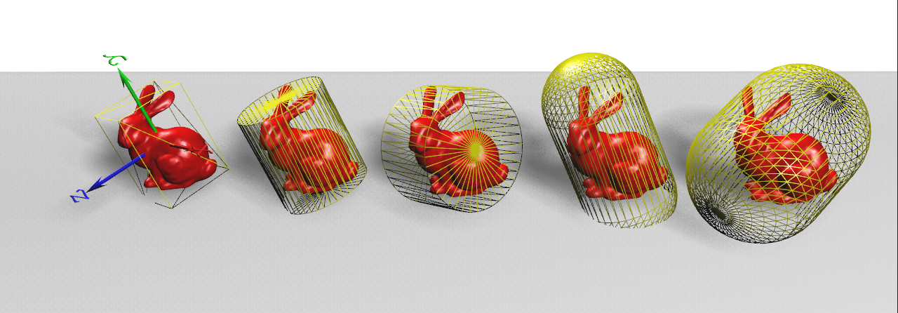
Fig. 12.6 This figure show a number of alternative bounding volumes and selection of principal axis for the computed shape.

12.7.12. WireShape

The wire shape is used internally for the collision handling of wire segments. It is based on the capsule, but might in the future have support for continuous collision detection. It is not advised to use this shape for other purposes, since implementation details might change.

12.7.13. HeightField

A height field is a geometric representation that can be used for terrain, sea beds etc. Height-fields are currently implemented as a scaled uniform grid centered at the local origin in x and y, and with z up. Furthermore, height-fields are treated like triangle meshes, where each rectangular grid cell is divided into a lower left and an upper right triangle. The corresponding class agxCollide::HeightField shares a common base class called agxCollide::Mesh with another mesh-based collision shape called agxCollide::Trimesh.

Compared to a trimesh, a height-field for collision detection as a terrain has the advantage of being able to modify the terrain under run-time. Trimeshes as terrains, on the other hand, can be modeled with fewer triangles by adapting the level of detail to the local change in terrain height, so that large plain parts can be covered by few large triangles.

Since trimeshes and height-fields share many routines for mesh traversal, please look into the trimesh chapter (12.7.9) for more information about that.

Fig. 12.7 HeightField representing uneven surface.

Like trimeshes used as terrains, height-fields make use of a bottom margin in order to have a safeguard in case objects tunnel downwards in local z-direction through the triangle surface.

12.7.13.1. HeightField creation

The height values in a height field can either be specified through a call to agxCollide::HeightField::setHeights() which accepts a vector in row matrix order or via a agxUtil::HeightFieldGenerator(), which can read data from an image (.png) or a raw binary file (no endian handling supported).

HeightField(size_t resolutionX, size_t resolutionY, agx::Real sizeX, agx::Real sizeY, agx::Real bottomMargin=agx::Real(1));

12.7.13.2. Modifying parts of a HeightField

The height values in a height field can also be changed in only a part of the whole shape. One possibility is by calling a version of agxCollide::HeightField::setHeights() which specifies which rectangular part of the grid to modify.

bool setHeights(const agx::RealVector& heights,
      size_t minVertexX, size_t maxVertexX, size_t minVertexY, size_t maxVertexY);

Another possibility is to set heights at specific points in the grid using the function agxCollide::HeightField::setHeight().

void setHeight(size_t xIndex, size_t yIndex, agx::Real height);

Note that all triangles around a changed height have to be updated. This update includes a recalculation of the triangle normal, as well as an update of the bounding volume hierarchy. Changing a single height will involve 6 updated triangles. Changing several heights within a rectangle can be done faster by using agxCollide::HeightField::setHeights() rather than agxCollide::HeightField::setHeight(), since this makes it unnecessary to update triangles several times.

12.7.13.3. HeightFields for dynamic simulation

There can be cases where it is of interest to combine the ease of modification of a height field with dynamical simulation, by making the height field part of the collision detection representation of an agx::RigidBody which is simulated dynamically. Since height-fields are generally assumed to be part of the static scenery, their mass properties are not calculated in the general case, since this comes with some computational cost. In order to get the mass-properties updated for dynamic simulation, call the method agxCollide::HeightField::setDynamic().

In order to compute these, a sort of box-shape is assumed for the height-field, where the top has a relief defined by the heights, the sides go downwards at the borders of the grid, and the bottom is a rectangle parallel to the z plane at a position given by a specified minimum height. To specify this height, use agxCollide::HeightField::setMinAllowedHeight().

Note that when changing parts of the height-field, the mass properties will not be updated. Instead, once all the updates are done and the new mass properties are needed for dynamic simulation, one should call agxCollide::HeightField:: calculateMassProperties() which will recalculate the mass properties for the whole height-field and can potentially be costly. This might be optimized in a future release.

12.7.14. Mesh reader

The class agxIO::MeshReader is capable of reading a number of 3D Mesh formats into mesh data that can be used to create a Trimesh or Convex shapes for collision detection. The enum agxIO::MeshReader::FileExtension lists all available formats. Most of the readers (with an exception to .shl) are utilizing the (Open Asset Importer Library) library for parsing the mesh files.

Note

Currently the MeshReader will concatenate all meshes into one mesh.

Table 12.3 Supported 3D Mesh model formats

File extension	Description
obj	Wavefront Obj
shl	Shell data format
fbx	Filmbox AutoDesk
assimp	AssImp reader/writer
dae	Collada
blend	Blender 3D
3ds	3ds Max 3DS
ase	3ds Max ASE
gltfb	Binary GL Transmission format
gltf	Ascii GL Transmission format
xgl	XGL
zgl	ZGL
ply	Stanford Polygon Library
dxf	AutoCAD DXF
lwo	LightWave
lws	LightWave Scene
lxo	Modo
stl	Stereolithography
x	DirectX X
ac	AC3D
ms3d	Milkshape 3D
scn	TrueSpace
xml	Ogre XML
irrmesh	Irrlicht Mesh
irr	Irrlicht Scene
mdl	Quake I
md2	Quake II
md3	Quake III Mesh
pk3	Quake III Map/BSP
md5	Doom 3
smd	Valve Model
m3	Starcraft II M3
unreal3d	Unreal
q3d	Quick3D
off	Object File Format
ter	Terragen Terrain
ifc	Industry Foundation Classes (IFC/Step)
ogex	Open Game Engine Exchange(.ogex)

12.7.15. Composite Shapes

Composite geometries are geometries containing more than one Shape. This can be useful when building more complex geometries from primitives.

There are basically two ways of creating a more complex Geometry structure around a rigid body.

1. Create a geometry g1, add shapes with relative transformations that builds up the final geometry. This also means that g1 can have only one material. (Material is bound per Geometry). Then, create a body b1 and add the created composite geometry g1.

2. Create a body b1, create the geometries needed g1, g2, … and for each geometry add shapes (Box, Sphere, …). Then, add each geometry to the body. In this case each geometry g1, g2… can each have different materials.

Note

There are two limitations when using composite shapes:

• If the single shapes forming the composite shape do not overlap, interacting objects might get in between them exactly where they touch. This might happen since the single shapes which the composite shape consists of do not know about each other. Therefore it is recommendable to let shapes overlap.

• However, when having overlapping shapes, the automatic mass property computation will count the overlapping volume twice. So here, manual mass property computation has to be used.

12.8. Shape colliders

A shape collider is a class that is responsible for calculating contact data between two shapes. The table below shows the available shapes and for which pair of shapes the AGX collision engine currently can calculate contact data.

12.8.1. Collider Matrix

In the following table, an overview over the functionality of colliders for different shape combinations is given. Reduced functionality means that basic functionality is given, but might have to be improved in the future in order to work perfectly in all purposes. Plane and HeightField make only sense as static geometries and can therefore not collide with themselves/each other.

Table 12.4 Available primitive tests

	Box	Capsule	Convex	Cylinder	Line	Plane	Sphere	Trimesh	Composite	HeightField	Cone	HollowCone	HollowCylinder
Box	X	X	X	X	X	X	X	X	X	X	(×)	(×)	(×)
Capsule	X	X	X	X	X	X	X	X	X	X	(×)	(×)	(×)
Convex	X	X	X	X	X	X	X	X	X	X	(×)	(×)	(×)
Cylinder	X	X	X	X	X	X	X	X	X	X	X	X	X
Line	X	X	X	X	X	X	X	X	X	X	X	(×)	(×)
Plane	X	X	X	X	X	—	X	X	X	—
Sphere	X	X	X	X	X	X	X	X	X	X	(×)	(×)	(×)
Trimesh	X	X	X	X	X	X	X	X	X	X
Composite	X	X	X	X	X	X	X	X	X	X	(×)	(×)	(×)
HeightField	X	X	X	X	X	—	X	X	X	—
Cone	(×)	(×)	(×)	X	X		(×)		(×)		X	X	X
HollowCone	(×)	(×)	(×)	X	(×)		(×)		(×)		X	X	X
HollowCylinder	[×]	[×]	(×)	X	(×)	[×]	[×]	[×]	(×)	[×]	X	X	X

The symbols in table 12.4 indicate: × Full functionality, (×) Reduced functionality, [x] using cylinder collider — Not needed (since both are supposed to be static).

12.8.2. Point, normal and depth calculation

In case of an intersection between two shapes, a shape collider will report one or more contact points. Each contact point consists of

• A point p,

• a normal n,

• a depth d.

The normal n points in the direction which lets shape1 move out of shape2.

The depth d measures how much shape 1 would have to be moved out of shape2 along normal n in order to resolve the overlap and thus have the two shapes just touching.

The point p is placed halfway between the two points corresponding to the surfaces of the two shapes, so that \(p_{shape_1 } = p- n * d * 0.5\) and \(p_{shape_2 } = p+ n * d * 0.5\).

12.8.3. Results for contacts with Line Shapes

The Line Shape is special in that its use is not in rigid body simulation, but in other fields as e.g. mouse picking or depth computation for unknown geometries. Therefore, the computation of contact point, normal and depth differs from that of the other Shapes.

The Line Shape represents mathematically a line segment, defined by two points \(P_0\) and \(P_1\), which define the non-normalized Line direction \(d = P_1- P_0\).

The Line can thus be presented as: \(P_0+ t \ d,0 \le t \le 1\).

If a Line intersects a Shape, the first point in contact \(P_c\) along the infinite version of the line is reported as contact point. The Shape surface normal is reported as contact normal. The parameter \(t_c\) is the value which realizes \(P_c= P_0+ t_c d\).

The depth is \((1 - t_c )*|P_0-P_1 |;\) this corresponds to how long the Line has to be pushed back in its direction in order to just touch the overlap point \(P_c\).

Exceptions:

• For mesh-based shapes (Trimesh, HeightField and at the moment also Convex), lines which are completely inside the shape will not create any contact.

• The line-line collider will create one contact point with a normal which is orthogonal to both lines and a depth of 0.

12.9. Storing renderable data in shapes: agxCollide::RenderData

agxCollide::RenderData is a class which can be used for storing renderable data together with a shape.

// Create a RenderData object
agxCollide::RenderDataRef renderData = new agxCollide::RenderData;

// Specify the vertices
agx::Vec3Vector vertices;
renderData->setVertexArray( vertices );

// Specify the normals
agx::Vec3Vector normals;
renderData->setNormalArray( normals );

// Specify the indices, which constructs Triangles
agx::UInt32Vector indices;
renderData->setIndexArray( indices, agxCollide::RenderData::TRIANGLES);

// Store a diffuse color
renderData->setDiffuseColor( agx::Vec4(1,0,1,1) );

This data can then be associated with an agxCollide::Shape:

gxCollide::ShapeRef shape = new agxCollide::Sphere(1.0);
shape->setRenderData( renderData );

During serialization to disk, this data will also be stored together with a shape. Later it can be retrieved with the call:

agxCollide::RenderData *renderData = shape->getRenderData();

In the sample coupling to OpenSceneGraph, agxOSG namespace, the function agxOSG::createVisual( geometry, agxOSG::Group *) will parse this render data and create a visual representation based on the RenderData (if available), otherwise it will use the specified shape when the renderable data is created.

12.10. Mass Properties

agx::MassProperty is a class which stores and handles the mass properties of a rigid body namely the heavy and effective mass of a rigid body. Whenever Geometries are added/removed to/from a rigid body with the methods

RigidBody::add(Geometry*)
RigidBody::remove(Geometry*),

the inertia tensor is recalculated by default, unless a previous call to RigidBody::getMassProperties()::setAutoGenerate( false ) has been done. In this case the inertia tensor and masses will NOT be updated when geometries are added and removed.

Attention

Currently, automatic mass property calculation (incremental or not) assumes all geometries and shapes to be disjoint (non-overlapping). If they overlap, the effect of this assumption is that the overlapping volume will be counted twice into mass and inertia computation. It is recommended to set the mass properties manually in this case.

An explicit inertia tensor can also be specified manually with the call:

body->getMassProperties()->setInertiaTensor(I);

where I can either be a SPDMatrix3x3 (semi positive definite) matrix or a Vec3 specifying the diagonal elements of the inertia tensor.

The method MassProperties::setInertiaTensor has a second parameter specifying whether the inertia tensor should be automatically recalculated, when set to false, the Inertia tensor for a rigid body will not be updated to reflect changes in associated Geometries.

During the calculation of mass properties, the density from the specified materials (described later) will be used to calculate the final mass. If no mass is specified explicitly for the body, the calculated mass will be used. If on the other hand the mass have been set by the user with the method RigidBody::getMassProperties()::setMass(), this mass will be used for the final result.

Unless the setAutoGenerate method has been called for a rigid body, the center of mass and inertia tensor will be updated for most operations such as adding/removing geometries, removing shapes from geometries. However there are a number of operations that will NOT be detected, and hence the user has to tell the body to update its mass properties:

• Transforming geometries relative the body after they are added to the body.

• Changing material properties (density) for any geometry added to a body.

• Transforming shapes that is part of a geometry associated to a body.

In the above cases the mass properties can be updated with a call to:

agx::RigidBody::updateMassProperties(agx::MassProperties::AUTO_GENERATE_ALL);

If you only want to update the inertia tensor you can change the argument to updateMassProperties. For more information see the SDK documentation.

12.11. Adding user forces

The class agx::RigidBody has the following methods for adding forces and torques:

addForce(), addForceAtPosition(), addForceAtLocalPosition(), addTorque().

These added forces are cleared after a time step has been taken in the simulation. The force added to a rigid body during the last timestep (including the forces introduced by the user via addForce/addForceAtPosition/addTorque , or via force fields etc. – however, NOT the ones from contacts and constraints!) can be accessed with the methods: RigidBody::getLastForce()/getLastTorque()

12.12. ForceFields

The class agx::ForceField can be used to induce user forces on all or a selected part of the bodies in a DynamicsSystem. It is derived from agx::Interaction.

#include <agx/ForceField.h>
class MyForceField : public agx::ForceField
{
  public:
  MyForceField() {}
  ~MyForceField() {}

  // Implement this method to add forces/torques of all or selected bodies
  void updateForce( DynamicsSystem *system );
};

// Create the force field and add to the DynamicsSystem.
agx::InteractionRef forceField = new MyForceField;
simulation->getDynamicsSystem()->add( forceField );

For a more thorough example, see tutorial_bodies.cpp in <agx>/tutorials/agxOSG/tutorial_bodies.cpp

12.13. GravityField

Gravitational forces should be applied through an instance of an agx::GravityField. The reason for this is that certain mechanics inside for example the wire implementation (agxWire::Wire) needs to know the individual gravity for each body.

By default, an instance of a class agx::UniformGravityField is created in DynamicsSystem, with the default acceleration of G = 9.80665 m/s². Another gravitational model is agx::PointGravityField, which will add a force towards a specified origin point. This model can be used for simulating the gravity on the surface of the earth.

To register a gravity field with the simulation the following call is done:

agxSDK::SimulationRef sim = new agxSDK::Simulation;
sim->setGravityField( new agx::PointGravityField );

Simulation::setUniformGravity and Simulation::getUniformGravity are just wrapper methods to simplify the use of the standard uniform gravity. A call to Simulation::setUniformGravity() will return false if the current gravity field model is not a agx::UniformGravityField.

12.13.1. CustomGravityField

The standard gravity fields (UniformGravityField and PointGravityField) are implemented as computational kernels to achieve best possible performance. However, to implement a custom gravity field, it is possible to derive from the class agx::CustomGravityField and implement the virtual method calculateGravity. The overhead compared to the standard gravity fields is the call to virtual method which should be small.

It is however important to remember that the method calculateGravity() will be called simultaneously from several threads if AGX is using more than one thread. This means that the method must be made thread safe.

class MyGravityField : public agx::CustomGravityField
{
public:
  MyGravityField() {}
  /// overidden method to calculate the gravity for a point in 3D Space
  virtual agx::Vec3 calculateGravity(const agx::Vec3& position) const
  {
    return position*-1;
  }
protected:
  ~MyGravityField() {}

};

// Register the gravity field with the simulation
simulation->setGravityField( new MyGravityField() );

12.14. Material

The material of a geometry will define how the geometry will get affected and affect the rest of the system. A material contains definitions of friction, restitution, density and other parameters that describe the physical surface, bulk and line attributes of a material. A material can be associated to a geometry with the method:

agxCollide::Geometry::setMaterial(agx::Material*)

An important thing to remember is that the name of a material has to be unique. Adding two materials with the same name will result in that only the first will be used in the system.

New materials must be registered with the agxSDK::MaterialManager before they can be used in the simulation (which is done when the material is added to the simulation).

When two geometries collide, the resulting contact parameters from the two involved materials are derived into an agx::ContactMaterial. The default contact material function can be overridden by adding explicit contact materials to the material manager.

Materials consist of three sub-classes which can be accessed through the calls:

material->getSurfaceMaterial();
material->getBulkMaterial();
material->geWireMaterial();

To complement the Material API, AGX also contains a Material Library with some predefined material properties that can be loaded and used as a starting point when designing simulations. See further in the Material Library section.

12.14.1. SurfaceMaterial

This class defines the behavior/surface attributes for contacts between geometries using two materials. The attributes currently available are:

• Roughness – Corresponds to friction coefficient, the higher value, the higher friction.

• Adhesion – determines a force used for keeping colliding objects together.

• Viscosity – Defines the compliance for friction constraints. It defines how “wet” a surface is.

• ContactReduction - Specifies whether contact reduction should be enabled for this material.

12.14.1.1. Roughness

The roughness describe what potential friction this material would have when it interacts with another material. The exact friction coefficient is calculated for the implicit contact material using the following equation: \(friction=\sqrt(roughness_1 \times roughness_2)\)

12.14.1.2. Adhesion

Adhesion defines an attractive force that can simulate stickiness. It operates only on bodies that have colliding geometries, i.e. it is not a general force field.

Adhesion is set using two parameters:

SurfaceMaterial::setAdhesion( adhesionForce, adhesiveOverlap );

adhesionForce specifies a force >=0, that is an upper bound of the attractive force acting between two colliding rigid bodies in the normal direction.

adhesiveOverlap is an absolute distance that defines the contact overlap where the adhesive force is active. Because that the adhesive force only acts upon overlapping rigid bodies, it is important to specify an overlap > 0. Otherwise a separating force would immediately (within a timestep) cause two bodies to separate, hence no adhesive force would then act on the bodies. The adhesiveOverlap is a safe zone to ensure that there will be time for the adhesiveForce to act.

Because the adhesive force operates only in the normal direction of the contact, it is also important to increase the roughness/friction to get a sticky behavior also in the friction direction.

\(max\_adhesive\_force \approx adhesiveOverlap / contact\_compliance\)

The adhesion distance will change the depth of the resting contact as seen in Fig. 12.8:.

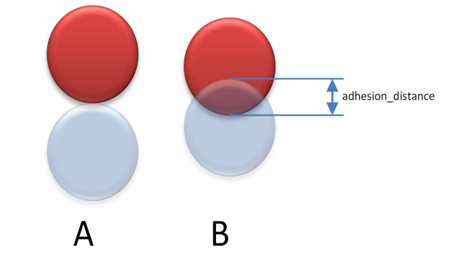
Fig. 12.8 A: no adhesion. B: adhesion_distance=r/2

The resulting adhesion parameters of an implicit contact material is calculated as \((adhesion_1+adhesion_2, min(adhesiveOverlap_1,adhesiveOverlap_2)\)

12.14.1.3. Surface viscosity

The viscosity of a surface material is the same thing as compliance but for friction in contacts. The resulting viscosity of an implicit contact material is calculated as \(viscosity = viscosity_1 + viscosity_2\)

12.14.1.4. Contact Reduction

This parameter specifies whether contact reduction should be enabled for this material. If two geometries overlap, the resulting contact material will get contact reduction enabled only if both materials have contact reduction enabled (logical and).

12.14.2. BulkMaterial

This class defines the density and other internal attributes of a simulated object. Lines use for example YoungsModulus and PoissonsRatio to calculate bending stiffness etc.

Attributes are:

• Density

• YoungsModulus – Stiffness of the material. Used when calculating contacts and the bending behavior of lines.

• Viscosity – Used for calculating restitution.

• Damping – Used for controlling how much time it should take to restore the collision penetration. A larger value will result in “softer” contacts.

12.14.2.1. Density

The density is used for calculating the mass of the rigid body from the volume of the geometry.

12.14.2.2. YoungsModulus

This specifies the stiffness of the contact between two interacting geometries/bodies. The resulting stiffness/young’s modulus for an implicit contact material is calculated as \((Y_1 \times Y_2) \div (Y_1 + Y_2)\)

12.14.2.3. Bulk viscosity

This defines the “bounciness” of an object or restitution in the contact material. The resulting restitution of an implicit contact material is calculated as \(restitution=\sqrt((1-viscosity_1)\times(1-viscosity_2))\)

12.14.2.4. Damping

This defines the time it should take for the solver to restore an overlap. A higher value will lead to higher restoration forces as overlaps should be minimized faster. The resulting damping of an implicit contact material is calculated as \(damping = max(damping_1, damping_2)\)

12.14.3. WireMaterial

Defines the behavior when a geometry with this material collides with a wire. Determines the stick and slide friction. When a wire is colliding with a geometry (where the wire is overlapping an edge of a box/trimesh, or onto a cylinder), a ShapeContactNode is created. This node is allowed to slide along the edge and also in the direction along the wire. To solve for the normal force, a 1D solver will analyze the system and solve how the contact node is allowed to move, depending on masses, gravity, physical properties in the wire and the tension in the wire.

Damping and Young’s Modulus can be specified for two attributes in the wire material:

• Bend – Constraint which tries to straighten a wire.

• Stretch - Constraint which works against stretching the wire.

For more information, see the SDK documentation on Material.

12.14.4. ContactMaterial

The class agx::ContactMaterial is used by the system to derive the actual material attributes when two materials collide. It can also be used to explicitly define a material used at contact calculations. All attributes found in the surface, bulk and line material is represented in the ContactMaterial, which is later used by the solver.

AGX use by default a contact point based method for calculating the corresponding response between two overlapping geometries.

There is also a different method available which is named area contact approach. This method will try to calculate the spanning area between the overlapping contact point. This can result in a better approximation of the actual overlapping volume and the stiffness in the response (contact constraint).

In general, this will lead to slightly less stiff, more realistic contacts and therefore the Young’s modulus value usually has to be increased to get a similar simulation results as running the simulation without the contact area approach.

// Create a contact material based on two agx::Material’s m1 and m2
agx::ContactMaterial *cm = simulation->getOrCreateContactMaterial(m1, m2);

// When two geometries collide, where m1 and m2 is involved, the contact area approach
// will be used.
cm->setUseContactAreaApproach( true );

agx::Real minElasticRestLength=0.0005, agx::Real maxElasticRestLength=0.05;
cm->setMinMaxElasticRestLength(minElasticRestLength, maxElasticRestLength);

The above code line determines the contact depth-span in which the material is elastic. AGX calculates this distance, but the material settings will put limits on this value. It can not be less than the minimum material rest length or greater than the maximum material rest length. For this reason, the minimum material rest length can not be greater than the maximum material rest length. For the theory background, see Contact mechanics (Elastic Foundation Model).

12.15. Calculating contact friction

At present, there is no difference between static and kinetic friction coefficients. According to published data and common models, these two coefficients differ by 10-20%. This is relevant in simulation of gear dynamics but not in most other cases. Friction coefficients do depend on the two materials in contacts.

So given material1 with roughness 0.5 and material2 with roughness 0.2, what friction coefficient should be used when these two materials get in contact? There is no clear picture of how to calculate this resulting friction coefficient in the general case. Therefore, by default, the resulting friction when material1 and material2 collides will be the geometric averaged value:

sqrt(material1.roughness*material2.roughness) = 0.31623

This is of course a crude approximation which does not have any relation to the real world physics. To overcome this, AGX supports explicit ContactMaterial, see Section 12.15.2.

Contacts are handled in two separate stages, namely, impact, and resting contact. Impacts correspond to a rigid body which is found in geometric interference at the beginning of a step with sufficiently large incident velocity, i.e., when the relative velocity projected on the separating normal is sufficiently negative. During impact resolution, the impacting energy is approximately restituted to the level of the restitution coefficient. This is done by computing an impulsive stage which preserves all constraints but applies a Newton restitution model on impacting contacts, with post impact velocity a fraction of the pre-impact incident velocity. That fraction is the restitution coefficient and it is usually a number between 0 and 1. The restitution coefficient applies to all pairs of rigid bodies and is part of the pair-wise contact properties. Because we do not locate the exact time of impact, there can be a small decrease in energy even if restitution is exactly 1.

After impact, constraint regularization and stabilization come into play. From the modeling perspective, this is no more and no less than a spring/damper system. Numerically, the spring and damper system is unconditionally for nonzero damping. The two parameters are accessible as contact compliance (1/YoungsModulus) and damping coefficient in the material properties. Compliance is just the inverse of the desired spring constant, with the usual units. The AGX damping parameter (also called “Spook damping parameter”) has units of time for technical reasons. Use the functions in agxUtil::Convert in order to convert from viscous damping coefficient to AGX’ damping coefficient.

There are basically two ways of setting up the material table for a complete system: defining implicit or explicit material properties.

12.15.1. Defining implicit Material properties

By creating an agx::Material, setting the properties, assigning it to a geometry and adding it to the Simulation, we have told the system that this geometry is created from some kind of material. When this geometry collides with another geometry, the pair of materials are used to calculate the resulting agx::ContactMaterial. This is a fairly easy way of creating the materials in the system, as every pair of materials does not really have to be known in beforehand. The calculation of material properties for the implicit contact material cm between material m1 and m2 is done as follows:

• cm.surfaceFrictionCoefficient = sqrt(m1.roughness*m2.roughness)

• cm.restitution = sqrt((1-m1.viscosity) * (1-m2.viscosity))

• cm.adhesion = m1.adhesion+m2.adhesion

• cm.youngsModulus = m1.youngsModulus * m2.youngsModulus / ( m1.youngsModulus + m2.youngsModulus )

• cm.damping = max(m1.damping, m2.damping)

• cm.surfaceViscosity = m1.surfaceViscosity+m2.surfaceViscosity

The frictional parameters for wire friction are using the same geometric medium as surface friction.

Note

We recommend that explicit contact material are used. This will give a better control over the simulation result instead of relying on the automatically calculated values in an implicit contact material.

12.15.2. Defining explicit ContactMaterial properties

If the actual values used in the friction solver has to be known exactly, the above method is not appropriate. Instead an explicit material table should be created.

This can be done by associating two agx::Material, M1 and M2 to one user created agx::ContactMaterial CM. So whenever the two materials M1 and M2 are involved in a contact, the attributes of CM are used. However, the following attributes of M1 and M2 still have to be set, to correctly calculate the mass properties of a RigidBody and to have correct behavior for LineConstraints.

BulkMaterial::setDensity()
BulkMaterial::setYoungsModulus()

At contact between two agx::Material’s the following list of attributes are used and should therefore be set to the required value.

ContactMaterial::setRestitution()
ContactMaterial::setFrictionCoefficient()
ContactMaterial::setLineStickFriction()
ContactMaterial::setLineSlideFriction()
ContactMaterial::setDamping()
ContactMaterial::setEnableContactReduction()

FRICTION	PLASTIC	METAL	WOOD
Plastic	??	0.7	0.3
Metal	—	??	0.2
Wood	—	—	??

Table showing friction coefficients between different materials, defined via explicit or implicit contact materials.

To build a table of explicit materials each ContactMaterial are associated to two agx::Material’s. Code for setting up this table could look like:

agx::MaterialRef wood = new agx::Material("Wood");
agx::MaterialRef plastic = new agx::Material("Plastic");
agx::MaterialRef metal = new agx::Material("Metal");

// Define the material for plastic/metal
agx::ContactMaterialRef plastic_metal = new agx::ContactMaterial(plastic, metal);
plastic_metal->setRestitution( 0.6 );
plastic_metal->setFrictionCoefficient( 0.7 );
plastic_metal->setYoungsModulus( 0.1E9 ); // GPa
// Define the material for wood/metal
agx::ContactMaterialRef wood_metal = new agx::ContactMaterial(wood, metal);
wood_metal->setRestitution( 0.2 );
wood_metal->setFrictionCoefficient( 0.2 );

// Define the material for wood/plastic
agx::ContactMaterialRef wood_plastic = new agx::ContactMaterial(wood, plastic);
wood_plastic->setRestitution( 0.4 );
wood_plastic->setFrictionCoefficient( 0.3 );
wood_plastic->setYoungsModulus( 3.654E9 ); // GPa

// Add ALL materials to the simulation
simulation->add(wood)
simulation->add(metal)
simulation->add(plastic)
simulation->add(plastic_metal);
simulation->add(wood_metal);
simulation->add(wood_plastic);

The above code example still leaves to the system to automatically derive the ContactMaterial for wood/wood, plastic/plastic and metal/metal.

12.15.2.1. ContactReduction

This parameter controls whether contact reduction should operate on the contacts where this contact material is used. For details, see Section 13.

12.15.2.2. Contact Area approach

If set to “true”, an approximation to the contact area will be geometrically computed for each contact involving this contact material. For each contact, its area will then be evenly distributed between its contact points. The contact compliance will be scaled with the inverse of the area for each contact point.

Note that this is an experimental feature, which has been tested on contacts involving meshes and boxes, but with a cruder approximation for contacts involving spheres or capsules.

Recommended for contact mechanics with a higher level of fidelity, such as grasping (involving meshes/boxes).

If set to “false”, unity area will be assumed (default).

// Define the material for wood/plastic
agx::ContactMaterialRef wood_plastic = new agx::ContactMaterial(wood, plastic);
wood_plastic->setUseContactAreaApproach(true);

12.15.3. Friction model

AGX has a hybrid solver which is very flexible in the way constraints can be configured. By default, contact constraints are solved in a split mode. This means that the normal force is solved in the direct solver and the friction is solved in the iterative solver. This behavior can be modified using ContactMaterials.

In the below examples, assume that the following code has been executed:

using namespace agx;
using namespace agxCollide;
// Create two materials
MaterialRef wood = new Material("wood");
MaterialRef steel = new Material("steel");

// Create two geometries with material steel and wood
GeometryRef geom1 = new Geometry;
geom1->setMaterial("wood");
GeometryRef geom2 = new Geometry;
geom2->setMaterial("steel");

// Create a contactmaterial that will be used when steel collides with wood
ContactMaterialRef steelWood = simulation->getMaterialManager()->getOrCreateContactMaterial( wood, steel );

12.15.3.1. BoxFriction

A naive implementation of this friction model will have static bounds through the solve stage. This means that for a stack of boxes, the bottom box, will not feel the weight of the other boxes. The normal force will be constant, as specified by the user. In our implementation we are estimating the normal force as follows:

• If the contact is now (i.e., new to the solver), the normal force is estimated by the impact (relative) speed.

• If the contact is old (i.e. created in a previous time step), the last normal force is used to set the bounds.

BoxFrictionModelRef boxFriction = new BoxFrictionModel();

// Use box friction as the friction model for this contact material
steelWood->setFrictionModel (boxFriction);

12.15.3.2. ScaledBoxFriction

The ScaledBoxFriction model gets callbacks from the NLMCP (Non-Linear Mixed Complimentary) solver with the current normal force. I.e., the correct normal force is used when setting the bounds. Scale box friction is computationally more expensive than the box friction but with a more realistic dry friction.

ScaledBoxFrictionModelRef scaledBoxFriction = new ScaledBoxFrictionModel();

// Use scaled box friction as the friction model for this contact material
steelWood->setFrictionModel (scaledBoxFriction);

12.15.3.3. IterativeProjectedConeFriction

This friction model is the default in AGX Dynamics.

When this method is used with Solve type SPLIT (which is default), it will split the the normal-tangential equations. I.e., the normal forces are first solved with a direct solve, and then both the normal and tangential equations are solved iteratively. For complex systems this could lead to viscous friction. This can be resolved by using DIRECT_AND_ITERATIVE solve model for other constraints (hinges, etc.) involved in the system. Iterative projected cone friction model is computationally cheap. Friction forces are projected onto the friction cone, i.e., you will always get friction_force = friction_coefficient * normal_force.

IterativeProjectedConeFrictionRef ipcFriction = new IterativeProjectedConeFriction();

// Use iterative projected cone friction as the friction model for this contact material
steelWood->setFrictionModel (ipcFriction);

12.15.3.4. Oriented friction models

Oriented friction models is of the same type as the ones described above but with the friction box/ellipse oriented with a given frame of reference and a primary friction direction (in the given frame).

const auto localPrimaryDirection = agx::Vec3::X_AXIS();
auto obfm = new agx::OrientedBoxFrictionModel( rb1->getFrame(),
                                               localPrimaryDirection );
auto osbfm = new agx::OrientedScaleBoxFrictionModel( rb2->getFrame(),
                                                     localPrimaryDirection );
auto oipcfm = new agx::OrientedIterativeProjectedConeFrictionModel( rb3->getFrame(),
                                                                    localPrimaryDirection );
cm1->setFrictionModel( obfm );
cm2->setFrictionModel( osbfm );
cm3->setFrictionModel( oipcfm );

Given a contact with an oriented friction model, the friction plane is calculated given the contact normal and the given primary friction direction. The secondary friction direction is orthogonal to the primary direction.

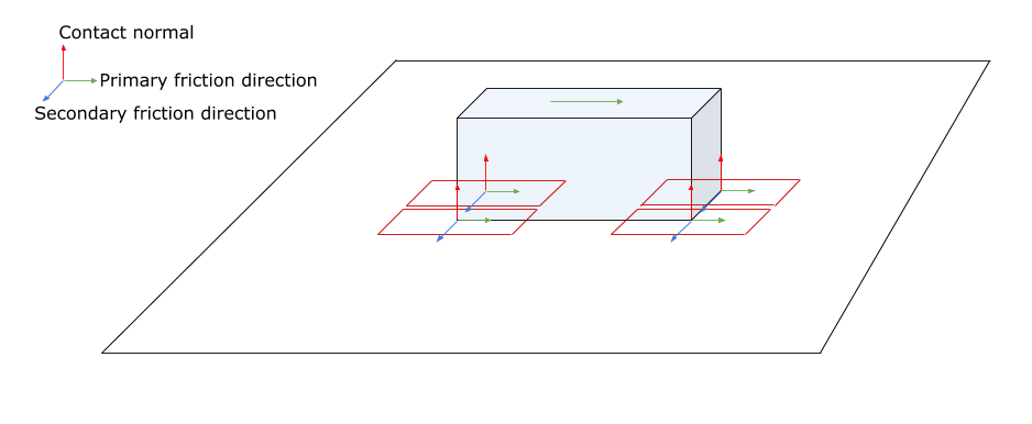
Fig. 12.9 Box with four contact points. The given primary direction (green arrows) orients the friction boxes.

12.15.3.5. ConstantNormalForceOrientedBoxFrictionModel

This friction model is similar to OrientedBoxFrictionModel but it has some additional features:

1. The normal force \(F_n\) is given, resulting in the primary friction force \(F_p\) to be bound by: \(-\mu_p F_n \leq F_p \leq \mu_p F_n\) and the secondary friction force \(F_s\) to be bound by: \(-\mu_s F_n \leq F_s \leq \mu_s F_n\) – where \(\mu_p\) is the primary friction coefficient and \(\mu_s\) the secondary friction coefficient.

2. Contact depth dependent maximum friction forces (disabled by default), by scaling the given normal force with the depth of each contact. Enabling this feature may impact the performance but the resulting behavior of the contacting objects may be better.

12.15.4. Solve type

As with any other constraint, we can also define how the normal/friction force will be solved:

FrictionModel::setSolveType (FrictionModel::SolveType solveType);

Table 12.6 Solve types for friction models

FrictionModel::SolveType	Description
DIRECT	Normal and friction equations are both solved in the DIRECT solver.
ITERATIVE	Normal and friction equations are both solved in the ITERATIVE solver.
SPLIT	Normal force solved in DIRECT solver, then normal and friction is solved in the ITERATIVE solver.
DIRECT_AND_ITERATIVE	Not recommended. Normal and friction are solved both in the direct and the iterative solver.

For an example of how to use the various contact solvers see Section 22.8.

12.15.4.1. DIRECT

In Section 3.4.2 the direct solver is described in more detail. Using the DIRECT solver for frictional contacts will allow very realistic friction simulation. It comes with a cost as the direct solver will generate NMLCP callbacks/iterations. For more information of how to achieve good performance see Section 40.

12.15.4.2. ITERATIVE

In Section 3.4.1 the iterative solver is described. The ITERATIVE solver is suitable for larger contact systems where the realistic contact friction can be traded against performance. It is usually a good idea to use the ITERATIVE solver together with agxSDK::MergeSplitHandler – AMOR, agx::MergedBody – many bodies simulated as one or AutoSleep to achieve fast and stable simulations.

12.15.4.3. SPLIT

The Split solver is the default contact solver. It balances performance with stability.

12.15.4.4. DIRECT_AND_ITERATIVE

This is not recommended and should be avoided.

12.16. Material Library

AGX contains some predefined material properties to help provide a starting point for the Material definitions in a simualtion. The definitions in the Material Library are generic, e.g. wood is defined, but not birch, oak or balsa tree. Those different types of wood have rather different properties, e.g. density. So for specific needs, the Materials used in a Simualtion should be defined according to your needs.

The definitions in the Material Library are limited to contain material properties and does not contain AGX implementation details. If for example a certain friction model is desired, then this has to be configured by the user.

When two materials from the material library interact, the material library is automatically searched for a predefined ContactMaterial for said Material pair. If none such ContactMaterial exists, then an implicit ContactMaterial is created and used.

The Material Library contains the following parts:

• Material definitions

• ContactMaterial definitiions

• TerrainMaterials

• BeamModelProperties

• CableProperties

Note

Some classes use more than just a Material for its definitions. Examples of this is e.g.

• agxCable::Cable which use both a Material and CableProperties,

• agxTerrain::Terrain which use Material and TerrainMaterial

• agxModel::BeamModel which use Material and BeamModelProperties

Example usage of the Material Library:

# Load into existing Material
my_material1 = agx.Material()
my_material1.loadLibraryMaterial("wood")

# Get a Material, None on failure
steel = agx.MaterialLibrary.loadMaterial("steel")

# Custom Materials can be based on items defined in the library
my_soft_steel = agx.Material(steel)
# customize my_soft_steel

# Modify the TerrainMaterial for a agxTerrain.Terrain
my_terrain.loadLibraryMaterial("dirt_1")

# Set both Material and CableProperties on a Cable:
my_cable.setMaterial(steel)
my_cable.loadLibraryProperties("cable_1")

# Some class based upon agxModel.BeamModel
my_i_beam.loadLibraryProperties("beam_1")

Classes that use properties have the method getAvailableLibraryProperties() whereas Terrain and Material have getAvailableLibraryMaterials() that can be used to inspect available items. This can also be done via agx::MaterialLibrary::getAvailableItems(item_type).

Which items that are available can also be seen by looking at the contents of <agx>/data/MaterialLibrary/<item type>/.

The different items are referenced by their short name. So for example if the Material steel is loaded, AGX searches for MaterialLibrary/Materials/steel.json. In the same way, if a CableProperty called cable_1 is requested, then the file MaterialLibrary/CableProperties/cable_1.json is search for. When a definition for a ContactMaterial is searched for, the name is the material1-material2 where the materials are in alphabetical order.

The lookup for all items in the material library is done using the RESOURCE_PATH and if you want to make AGX search at more locations, see Locating files with agxIO::Environment.

Note

GranularBodySystem settings in ContactMaterial

The ContactMaterial definitions all list default values used by the GranularBodySystem for GraularBody specific parameters such as rolling resistance and twisting resistance. The reason for this is to expose the values in case someone wants to define their own materials. These values are highly shape dependent and what the granulars look like have a much larger effect on the parameter values than the actual combination of materials that interact.

E.g. if the granulars that interact are spheres or boxes influence the values more than if it is wood-wood or wood-steel.

12.16.1. Adding new items to the Material Library

The material library can be extended locally if wanted. This is done by placing a json file in the corresponding MaterialLibrary/<item type>/ directory. Existing files can be used to see which parameters that should be defined.

When adding a Material there is one special value in the file that is important for how contact materials are found. That is the value for name. In the files provided with AGX Dynamics, the name value matches the filename, e.g. MaterialLibrary/Materials/wood.json have “name”: “wood”. It is the pair of two such names that are used when searching for a contact material when two library materials interact.

The reason for “name” is that one can have e.g. birch.json and pine.json and both use wood for name. Then interactions for the specific birch material would use the predefined contact materials that already exist for wood.

12.17. Testing user geometry against Space

In some cases it is of interest to intersect the current configuration in the collision space with some geometries, without actually inserting a new geometry into the collision space.

As soon as a geometry is inserted into space, it is a part of the simulation. Also testing for contacts in between two simulation frames can sometime be used for example for path finding etc.

There are two methods for achieving this in agxCollide::Space:

bool Space::testBoundingVolumeOverlap(
      agxCollide::GeometryPtrVector& testGeometries,
      agxCollide::GeometryPairVector& result,
     bool skip = true );

bool Space::testGeometryOverlap(
     agxCollide::GeometryPtrVector& testGeometries,
     agxCollide::GeometryContactVector& result,
     bool skip = true );

testBoundingVolumeOverlap will take a vector of Geometries and return pairs of Geometries with overlapping bounding volumes.

testGeometryOverlap will take a vector of Geometries and return a vector of geometry contacts, including contact points, penetration, normals etc. …

12.18. Reading forces from the simulation

Often when you build a simulation you also want to read forces/torques from the system. Assume you have built your scene with geometries, bodies, constraints and wires. Now how do you access the forces from your simulation?

Note: As in many parts of this documentation, the term “force” is here used interchangeably for a 3d force vector in contrast to a 3d torque vector and, where applicable, as a 6d vector consisting of both force and torque.

Forces can be divided into a few separate categories:

• External/ForceField/Gravity forces

• Constraint forces

• Contact forces

12.18.1. External/ForceField/Gravity forces

Forces and torques can be applied to a body by the methods:

RigidBody::addForce, RigidBody::addTorque, etc. see 12.11.

External forces also include forces added by ForceFields, GravityFields. These external forces can at any time be read from a given rigid body with the method:

const agx::Vec3& RigidBody::getLastForce() const;
const agx::Vec3& RigidBody::getLastTorque() const;

12.18.2. Constraint forces

It is possible to read constraint forces applied to rigid bodies during the last time step for each constraint. However, it is currently not possible to ask a rigid body for its constraint forces directly - you have to keep track of the constraints attached to a specific body yourself and ask those constraints for the forces.

12.18.2.1. Constraint::getLastForce per body

For computational reasons, the calculation of constraint forces is disabled by default. To enable the computation of constraint forces call the method:

void Constraint::setEnableComputeForces(bool);

once for each constraint that you want to read forces from in the future.

Then, after the solver has been executed, you can access (e.g. with a StepEventListener in POST) the forces/torques applied to the constrained bodies with a call to:

// If you know the index of your body in the Constraint (0 or 1)
bool Constraint::getLastForce( UInt bodyIndex, Vec3& retForce, Vec3& retTorque, bool giveTorqueAtCm=false ) const;

// If you have pointer to the rigid body
bool Constraint::getLastForce( const RigidBody* rb, Vec3& retForce, Vec3& retTorque, bool giveTorqueAtCm=false ) const;

Note that getLastForce is only valid when called for a rigid body with motion control DYNAMICS or KINEMATICS (not STATIC). Check the return value to detect invalid calls to getLastForce.

The returned force and torque by getLastForce are defined in the world coordinate system.

The returned torque depends on the value of the flag giveTorqueAtCm:

• A value of true gives the torque in the body’s center of mass (corresponding to RigidBody::addTorque(Vec3)),

• whereas the default value of false gives the value in the constraint’s attachment point r for the body, so that tau_attachment = tau_cm + r cross F

12.18.2.2. Constraint::getCurrentForce per constraint-DOF

If you are interested in obtaining the force applied by the constraint at a certain degree of freedom (in the constraint’s local coordinate system), you can use

// \return the current force magnitude (i.e., the force magnitude last time step) in given DOF >= 0 && <= NUM_DOFS
bool Constraint::getCurrentForce( UInt degreeOfFreedom) const;

Note that the degrees of freedom have different meanings for each constraint type; the enum DOF which is defined per constraint should be used.

The method getCurrentForce exists also for secondary constraints (see 15.12.5).

Attention

The naming difference in getCurrentForce and getLastForce is misleading since both methods read the forces from the same source and time. These methods will likely be renamed in the future to reflect their behavior better.

12.18.3. Contact forces

Contact forces are included in the contact data, together with contact points, normals depths, … . Contact forces are valid after the solver has been executed. You can access them (e.g. with a StepEventListener in POST) like in the following example.

Assume you want to collect the sum of the absolute values of all the contact forces (normal and friction) being applied on a specific rigid body:

#include <agxCollide/Contacts.h>
#include <agxCollide/Space.h>

// Return the sum of the magnitude for all contact forces being applied to a specific body.
agx::Real getContactForce(agx::RigidBody* body, agxCollide::Space* space)
{
  // Get the vector with all the contacts
  const agxCollide::GeometryContactPtrVector& contacts = space->getGeometryContacts();

  agx::Real contactForce = 0;
  // For all contacts in the system
  for (size_t i = 0; i < contacts.size(); ++i)
  {
    agxCollide::GeometryContact *gc = contacts[i];
    // Is the contact enabled?
    if (!gc->isEnabled())
      continue;
    // Is our body involved in this contact?
    if (gc->rigidBody(0) != body && gc->rigidBody(1) != body)
      continue;

    // Get all the points and sum the magnitude for the contact force (normal force)
    const agxCollide::ContactPointVector& points = gc->points();
    for (size_t n = 0; n < points.size(); ++n)
    {
      // Is the contact point enabled?
      if (!points[n].enabled())
        continue;
      contactForce += points[n].getNormalForceMagnitude();
    }
  }
  return contactForce;
}