19. AGX DriveTrain
agxDriveTrain is a library of AGX PowerLine components designed to model the various parts of a vehicle drive train. It deals exclusively with rotational motion, hence all components inherit either from RotationalUnit or from RotationalConnector.
To use components which are part of the PowerLine API one must first create a PowerLine instance to hold the components:
agxPowerLine::PowerLineRef powerLine = new agxPowerLine::PowerLine();
simulation->add(powerLine);
19.1. Shaft
The Shaft is the most basic drive train Unit. It is simply a rotating body that we can connect Connectors to.
agxDriveTrain::ShaftRef shaft1 = new agxDriveTrain::Shaft();
powerLine->add(shaft1);
19.2. Gear
The Gear is the most basic drive train Connector. It is used to transfer rotational motion between the Unit-based drive train components. A Gear is actually the interaction between two geared wheels, one from each connected Unit, and has therefore a gear ratio. The gear ratio define the number of gear teeth on the output shaft to the number on the input shaft. A gear ratio magnitude higher than 1 will cause the output gear to rotate slower than the input shaft, and a gear ratio magnitude lower than 1 will instead cause the output gear to rotate faster than the input shaft. Negative gear ratios make the output shaft rotate in the opposite direction of the input shaft.
where \(g\) is the gear ratio.
A pair of shafts are connected using code such as the following:
agxDriveTrain::ShaftRef shaft2 = new agxDriveTrain::Shaft();
agxDriveTrain::GearRef gear = new agxDriveTrain::Gear();

powerLine->add(shaft2);
powerLine->add(gear);

gear->setGearRatio(agx::Real(2.0));

shaft1->connect(gear);
gear->connect(shaft2);
With the system created so far, since shaft1 is the input of the gear and shaft2 is the output, whenever shaft1 is rotating, shaft2 will rotate at half the speed.
In addition to the basic Gear, there are other drive train components which have gear-like behavior.
19.2.1. GearBox
A gear box is a gear-like connector that has a collection of gear ratios that it can switch between. It is created from a vector of gear ratios and provides methods for changing the currently selected gear.
agx::RealVector gearRatios;
gearRatios.push_back(agx::Real(10));
gearRatios.push_back(agx::Real(7));
gearRatios.push_back(agx::Real(5));
gearRatios.push_back(agx::Real(3.5));
gearRatios.push_back(agx::Real(2));
gearRatios.push_back(agx::Real(1));
agxDriveTrain::GearBoxRef gearBox = new agxDriveTrain::GearBox(gearRatios);

gearBox->setGear(0);
The above example creates a gear box with six gears with decreasing gear ratios, i.e., increasing output shaft velocity, and set the current gear to the first one.
19.2.2. SlipGear
A gear with a configurable compliance. Increasing the compliance will cause the gear to slip more under load.
19.2.3. HolonomicGear
A regular Gear uses a nonholonomic constraint to maintain the velocity relationship, which means that small differences in angle may accumulate over time. The HolonomicGear uses a holonomic constraint instead, which ensures that the two connected shafts never slip.
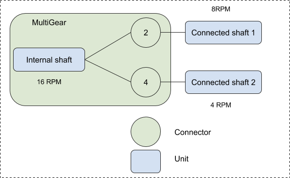
19.2.4. MultiGear
A gear that allows for multiple connected shafts, each with its own gear ratio. Whenever one of the connected shafts rotate a hidden internal shaft will rotate with a velocity corresponding to the gear ratio configured for that connected shaft. All other connected shafts will then rotate along with the internal shaft with the velocity that corresponds to their respective gear ratio.
A MultiGear only support connections on the output side.
19.2.5. TorqueConverter
The torque converter is a viscous coupling between two rotating axes. When there is a velocity ratio between the incoming shaft and the outgoing there will be a torque multiplication. The incoming shaft rotates a pump which accelerates a fluid. The fluid will accelerate a turbine which is connected to the outgoing shaft.
The torque converter is created simply as:
TorqueConverterRef tc = new TorqueConverter();
When the torque converter is created it is set up with default values, for what should be a generic torque converter. This means that after creating it, it can be connected to the drive train and used directly.
The torque converter contains a lock that can be enabled to lock it so it will have the same input and output velocities.
tc->enableLockUp(true);
This lock should be disabled when switching gear, suddenly increasing velocity or when braking.
19.2.5.1. Torque converter characteristics
The multiplication you get from a specific torque converter depends on the internal construction of the pump and the turbine. The torque converter has two important tables that define its behavior; the geometry factor table and the efficiency table.
The torque needed to rotate the pump is calulated using the geometry factor table, \(\xi(\nu)\), which depends on the velocity ratio between the turbine and the pump: \(\nu = \omega_{t} / \omega_{p}\). The pump torque is calculated as
where \(\rho\) is the fluid density and \(d_{p}\) the pump diameter, parameters that can also be modified to change the torque converter behavior. The geometry factor table can bet set with the following method:
TorqueConverter::setGeometryFactorTable(const agx::RealPairVector& velRatio_geometryFactor);
The efficiency table \(\psi(\nu)\) determines the amplification of the output torque on the turbine side. The torque is calculated as
The efficiency table can be set using this method:
TorqueConverter::setEfficiencyTable(const agx::RealPairVector& velRatio_efficiency);
19.3. Engine
An engine is a Unit that is a source of power in a drive train. There are three types of engines: torque curve based, fixed velocity based and the combustion engine.
19.3.1. Torque curve engines
Torque curve engines uses a torque curve to determine the maximum available torque for the current RPM and a user controlled throttle to select a fraction of that available torque to actually apply. The Engine class is a torque curve engine. It is used as follows:
agxDriveTrain::EngineRef engine = new agxDriveTrain::Engine();
agxPowerLine::PowerTimeIntegralLookupTable* torqueCurve =
    engine->getPowerGenerator()->getPowerTimeIntegralLookupTable();
torqueCurve->insertValue(rpm0, torque0);
torqueCurve->insertValue(rpm1, torque1);
torqueCurve->insertValue(rpmN, torqueN);
engine->setThrottle(throttle);
Every time step the engine does a lookup into the torque table to find the maximum available torque for the current RPM. It then scales the maximum torque with the current throttle, a value between 0 and 1, to find the torque to apply this time step. The engine uses piecewise linear interpolation for lookups between the inserted values, and extrapolation of the first two or last two values for lookups outside of the torque curve domain.
An Engine has an idle RPM and the power generator has a corresponding minimum torque. When the engine is below the idle RPM, then the power generator will apply at least the minimum torque to reach the idle RPM.
Another torque curve engine is the PidControlledEngine. It inherits from Engine and by default behaves almost the same. The added functionality it provides is an ignition used to start and stop the engine and the ability to control the throttle automatically, for example to maintain a target RPM. Specific throttle controllers are created by inheriting from ThrottleCalculator. Provided with agxDriveTrain is RpmController, which is a PID controller that tries to maintain a target RPM.
engine = new agxDriveTrain::PidControlledEngine();
controller = new agxDriveTrain::RpmController(engine, targetRpm, pGain, dGain, iGain, iRange);
engine->setThrottleCalculator(controller);
engine->ignition(true);
// Don't forget to create the torque curve as well.
Idle RPM works differently for a PidControlledEngine compared to the base Engine. If a ThrottleCalculator has been set then that has full control over the throttle. If a ThrottleCalculator has not been set then the PidControlledEngine will use setGradient to force the engine RPM to reach the idle RPM.
19.3.2. Fixed velocity engine
The fixed velocity engine uses a velocity constraint to maintain the target velocity. This type of engine can be used when the expected velocity of the engine is known and any amount of torque is allowed to reach that velocity.
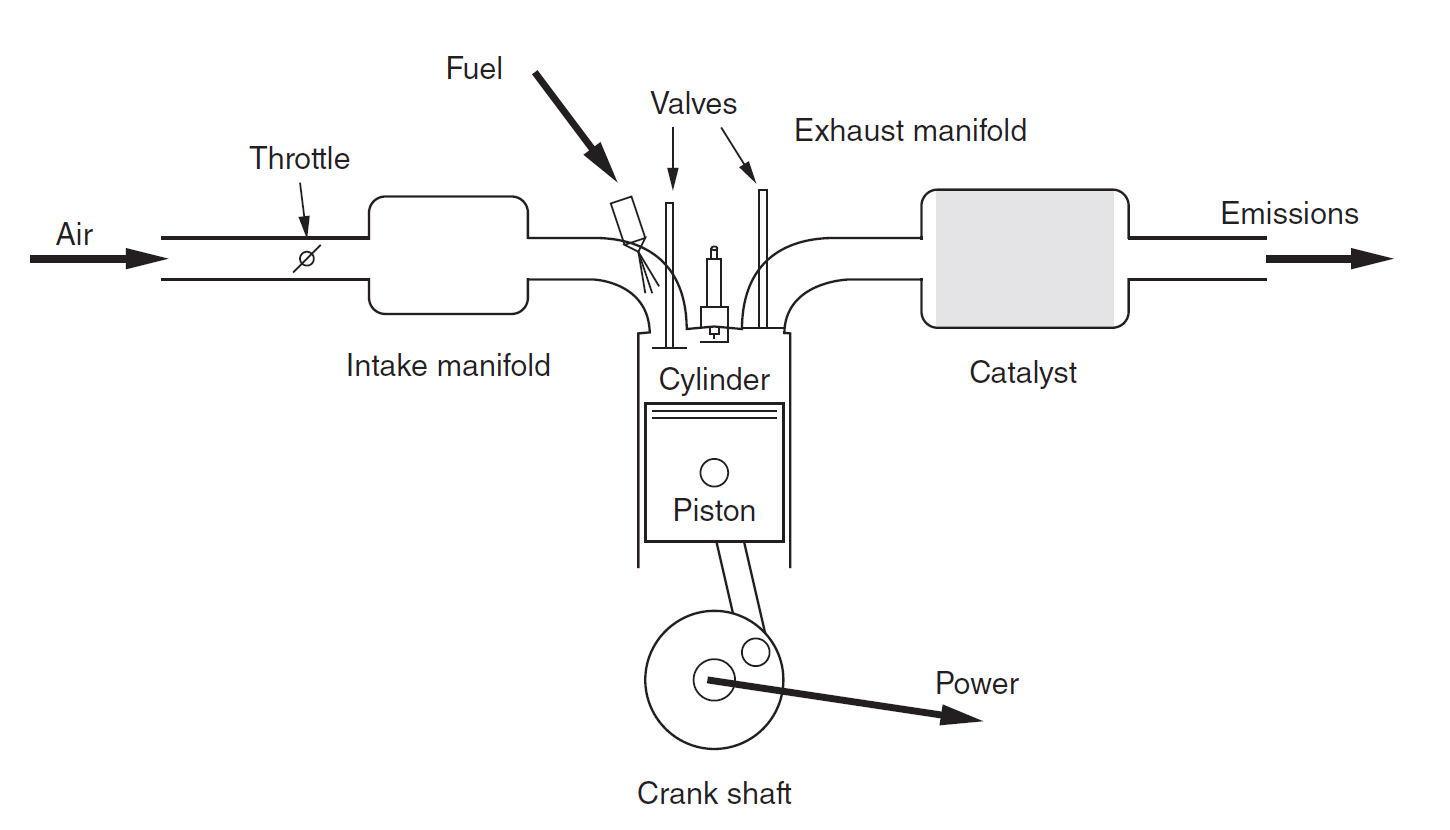
19.3.3. Combustion engine
Combustion engine [13] is one of the most widely used types of engines in various applications such as vehicles, excavators, wheelloaders, aircrafts and marine propulsion systems. It includes a number of components as shown in Fig. 19.1, such as the cylinders, pistons, crankshaft, camshafts, valves, fuel injection system, ignition system, air intake and exhaust systems. The cylinders and the pistons form the main body of the engine, where the combustion process occurs. The combustion converts the chemical energy of the air-fuel mixture into the heat energy. The heat energy generates the high temperature as well as the high pressure inside the cylinders. The pressure pushes the pistons to move during the power stroke and outputs the torque to rotate the crank shaft. The crank shaft drives the gears in the drive train, which eventually enables the motion of the vehicle. The valves control the flow of air and fuel into and out of the engine cylinders, and the fuel injection and ignition systems manage the combustion process.
As a critical component of the vehicle, it is important to model the combustion engine accurately since it directly affects the performance of the vehicle, such as the stability, handling, and ride comfort. A detailed engine model can provide information such as the engine speed, torque, power and the fuel consumption. This information is critical for the design and development of efficient power train systems as well as the effective controlling strategies of the vehicle. This contributes to the increasing demands of accurate and efficient combustion engine models.
Modelling of the combustion engine involves the use of mathematical equations that accurately represent the physical behavior of the engine such as the thermodynamics, fluid mechanics, and rotational dynamics. The thermodynamic properties of the air-fuel mixture determine the efficiency and power output of the engine, while the fluid mechanics determine the flow of air and fuel into the combustion chamber. The rotational dynmics are important for modelling the engine’s crankshaft and connecting rods, which convert the linear motion of th pistons into the rotational motion. Depending on the level of details required, the models of combustion engine can be simplified or complex. For instance, in [14], computational fluid dynamics (CFD) method, which solves the partial differential equations, is used to simulate the combustion process. In [15], the dynamic artificial neural networks (ANN) have been employed to develop an engine model with high accuracy.
19.3.3.1. Modelling theory
In AGX Dynamics, the mean value engine model (MVEM) [13] has been implemented to model the combustion engine. It is a simplified time-based model used to predict averaged key engine combustion variables without modeling the detailed physical combustion process. It captures the dominated combustion characteristics averaged over one or several engine cycles.
The governing equations of the MVEM theory are simply just two ordinary differential equations as listed below.
The first equation is formulated for the development of the intake manifold pressure \(p_{im}\). \(T_ {im}\) refers to intake temperature. \(V_{im}\) is the volume of the intake manifold. \(R\) is the specific gas constant. The mass difference between throttle inflow \(\dot{m}_{\text{at}}\) and cylinder outflow \(\dot{m}_{\text{ac}}\) directly gives the rate of mass change in the intake system. It is worth noting that this differential equation is derived from the ideal gas law \(pV = mRT\).
The second equation is formulated for the rotational dynamics of the engine crankshaft with the moment of inertia \(J\). \(N\) is the rotational speed of the crank shaft. \(M_i\) is the indicated torque, \(M_f\) is the friction torque consumed by the engine components, \(M_{p}\) is the pump torque, \(M_{load}\) is the output torque.
19.3.3.1.1. Throttle mass flow
The throttle air mass flow \(\dot{m}_{at}\) is dependent not only on the motion of the throttle plate but also on the pressure development in the intake manifold. It is expressed as [6],
where \(T_{\text{amb}}\) and \(p_{\text{amb}}\) are the ambient temperature and pressure, \(A_{\text{eff}}(\alpha)\) is the effective throttle openning area, \({\Psi_{\text{li}} \left( \Pi \left( \frac{p_{\text{im}}}{p_{\text{amb}}} \right) \right)}\) is the flow function. Here, the flow passing through the small throttle area has a large pressure difference, and the gas flow velocity is very high, which can be 70-100m/s. The flow is modelled as isentropic compressible flow.
19.3.3.1.2. Engine mass flow
The cylinder air mass flow \(\dot{m}_{ac}\) depends on the engine speed \(N\), intake pressure \(p_{im}\), and temperature \(T_{im}\). It is expressed as,
where the volumetric efficiency \(v_{vol}\) defines the engine’s capability to induct new air into the cylinders. \(v_{vol}\) is defined as [16]
where, \(c_{0}\), \(c_{1}\), \(c_{2}\), \(c_{3}\) are pressure- and engine-speed-related coefficients.
19.3.3.1.3. Engine torques
The indicated torque \(M_{i}\), the friction torque \(M_f\) and the pump torque \(M_p\) are calcualted as
where \(\dot{m}_{f}\) refers to the fuel flow rate, \(Q_{hv}\) is the heat value, \(\eta_{t}\) is the thermal efficiency, \(AF\) is the stoichiometric air-fuel ratio. \(C_{fr0}\), \(C_{fr1}\) and \(C_{fr2}\) are the coefficients [13] that define the quadratic relationships between friction torque \(M_{f}\) and engine speed \(N\). \(p_{em}\) is the pressure of the exhaust manifold.
Note
The default values of the torque friction parameters \(C_{fr0}(0.97)\), \(C_{fr1}(0.15)\) and \(C_{fr2}(0.04)\) are valid for engines with displacement volumes ranging from 0.845L to 2.0L according to [13]. For other engines, it is recommended to calibrate these parameters against real engine tests.
19.3.3.2. Build combustion engine
The combustion engine is parameterized, created and started in the example below:
agxDriveTrain::CombustionEngineParameters engineParameters;
agxDriveTrain::CombustionEngine::readLibraryProperties("Saab-B234i", engineParameters);
agxDriveTrain::CombustionEngineRef engine = new agxDriveTrain::CombustionEngine(engineParameters);
engine->setEnable(true);
Note that the combustion engine must be enabled to start it. Here, the program pre-set Saab engine with the displacement volume of 2.3 liter, the max torque of 212 Nm at 4000RPM is used.
An engine can be reconfigured after creation:
// Initialize the engine as a Saab B234i engine.
agxDriveTrain::CombustionEngine.readLibraryProperties("Saab-B234i");
agxDriveTrain::CombustionEngineRef engine = new agxDriveTrain::CombustionEngine(engineParameters);

// Reconfigure it as a Volvo T5.
engine->loadLibraryProperties("Volvo-T5");
engine->setEnable(true);
19.3.3.2.1. Engine Parameters
The data dictory in AGX Dynamics contains a set of pre-defined engine models in json data files. They can be located in <agx_dir>/data/MaterialLibrary/CombustionEngineParameters.
A parameter file can be adressed by its name, e.g. “Saab-B234i” or “Scania-K310UB4X2Euro5”. Each json file contains the CombustionEngineParameters as well as the torque friction coefficients.
New engines can be defined by copying one of the existing files and creating a new with different parameters.
Engine parameters can also be explicitly declared in code:
agxDriveTrain::CombustionEngineParameters engineParameters;
engineParameters.displacementVolume = 0.003;
engineParameters.maxTorque = 300;
engineParameters.maxTorqueRPM = 3000;
engineParameters.maxPowerRPM = 4000;
engineParameters.idleRPM = 1000;
engineParameters.maxRPM = 9000;
engineParameters.crankShaftInertia = 0.5;
agxDriveTrain::CombustionEngineRef engine = new agxDriveTrain::CombustionEngine(engineParameters);
engine->setEnable(true);
All the engine parameters that are needed for customizing a combustion engine are listed and described below.
Parameter |
Unit |
Description |
displacementVolume |
m^3 |
The total displacement volume of the engine, which is the sum of the volumes of the cylinders. |
maxTorque |
Nm |
The maximum rated torque which is the highest brake torque that an engine is allowed to deliver over short/continous periods of operations |
maxTorqueRPM |
RPM |
The rated torque speed (i.e. the crankshaft rotational speed) in which the maximum rated torque is delivered. |
maxPowerRPM |
RPM |
The rated power speed (i.e. the crankshaft rotational speed) in which the maximum rated power is delivered. |
idleRPM |
RPM |
The crankshaft speed in which the engine is at idle condition. |
maxRPM |
RPM |
The maximum allowerable crankshaft speed of the engine. |
crankShaftInertia |
kg m^2 |
The moment of inertia of the crank shaft. |
cfr0 |
Coefficients that define the quadratic relationships between friction torque and engine speed |
|
cfr1 |
Coefficients that define the quadratic relationships between friction torque and engine speed |
|
cfr2 |
Coefficients that define the quadratic relationships between friction torque and engine speed |
|
throttlePinBoreRatio |
Optional. Set the ratio between throttle pin diameter and throttle bore diameter |
|
maxVolumetricEfficiency |
Optional. Maximum volumetric efficiency of the engine. The volumetric efficiency refers to the ratio of air volume drawn into the cylinders to the volume the cylinder sweeps. |
|
airFuelRatio |
Optional. Set the stoichiometric air-fuel ratio. Ideal ratio of air to fuel needed for complete combustion, e.g. gasoline. |
|
heatValue |
J/kg. |
Optional. Set the heat value of the fuel |
nrRevolutionsPerCycle |
Optional. |
19.3.3.2.2. Throttle control
To change the velocity of the engine the throttle can be controlled. The value of the throttle is varying between 0 and 1, where 0 means idle and 1 full throttle.
engine->setThrottle(throttle);
The throttle parameters and throttle control methods are listed and described below. Also, the other engine parameters such as the number of revolution per cycle can be specified by the user given the varying engine configuration.
Parameter |
Method |
Description |
Throttle |
setThrottle |
Percentage of open throttle. Value between 0 and 1. |
Throttle Angle |
setThrottleAngle |
Set the angle of the throttle plate, instead of the percentage it is open |
Idle Throttle Angle |
setIdleThrottleAngle |
The minimum angle the throttle plate can have when engine is running |
Max. Throttle Angle |
setMaxThrottleAngle |
The maximum angle the throttle plate is allowed to open |
Detailed C++ and python examples with combustion engine are available
in tutorials/agxOSG/tutorial_driveTrain_combustionEngine.cpp,
tutorials/agxOSG/tutorial_driveTrain_torque_converter.cpp and
python/tutorials/tutorial_driveTrain_combustionEngine.agxPy.
19.3.3.3. Engine performance
Fig. 19.2 shows the torque/power curves of the combustion engine with the Saab engine parameters.
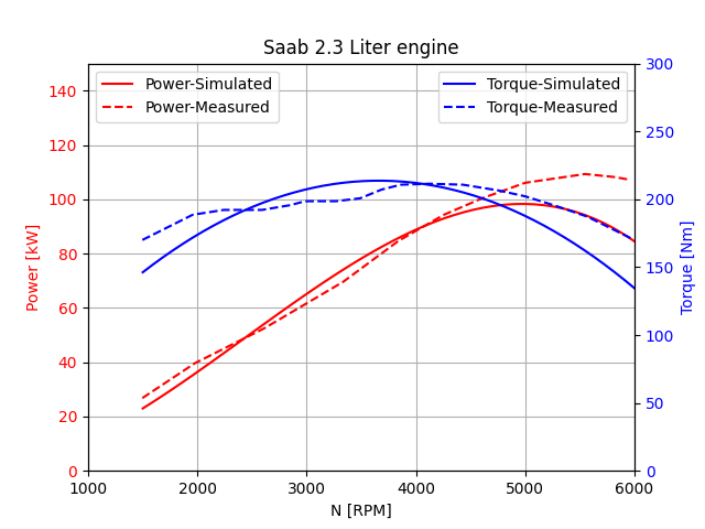
Fig. 19.2 Torque/power curves of Saab engine.
Fig. 19.3 shows the torque/power curves of the combustion engine with the Volvo excavator engine parameters.
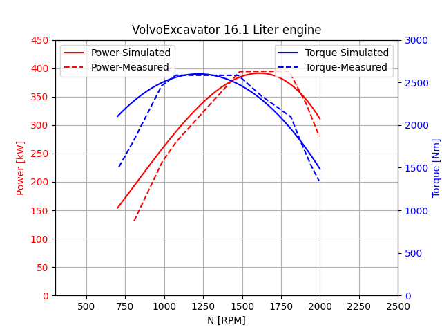
Fig. 19.3 Torque/power curves of volvo excavator engine.
19.4. Electric motor
An electric motor is a Unit that, similar to an engine, is a source of power in a drive train. It simulates the conversion of electrical energy to mechanical energy.
When creating an electrical motor one must first know the resistance, inductance, torque constant and back electromotive force (EMF) constant of the motor. The torque constant, \(\alpha\), is related to the torque, \(\tau\), and current, \(I\), as follows
The EMF constant, \(\beta\), is related to the back EMF, \(V\), and the angular velocity of the motor, \(\omega\), as follows
For an ideal motor \(\alpha = \beta\). However, if we have additional energy losses in the motor then \(\beta \leq \alpha\). This happens at high current since energy in the form of heat is dissipated in the armature of the motor, and we thus get less mechanical energy out than electrical energy in.
When the motor is created the input voltage to the motor is by default set to zero, and thus it must be set to some other value to start the motor.
agxDriveTrain::ElectricMotorRef motor = new agxDriveTrain::ElectricMotor( resistance, torqueConstant,
                                                                          emfConstant, inductance );
motor->setVoltage( voltage );
The voltage can be set at each time step to regulate the angular velocity of the motor.
19.5. Clutch (deprecated)
Note
The class Clutch has been deprecated and we recommend using dryclutch instead.
A clutch is a Connector with a configurable efficiency and torque transfer constant. The efficiency is a value between 0 and 1 where 0 means no torque transfer and 1 means a rigid coupling. The torque transfer constant define the shape of the torque transfer curve as the efficiency is changed between 0 and 1, where a larger constant leads to a faster increase in torque as the efficiency is increased.
19.6. DryClutch
Dry-clutch as shown in Fig. 19.4 a) is a mechanism that can connect and disconnect the engine from the rest of the transmission, without stalling the engine. This is done by compressing rough plates against each other, allowing them to slip during the engagement process.
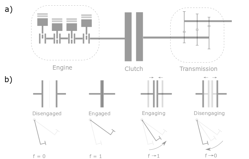
Fig. 19.4 Dry clutch schematic. a) Relative position; b) Working schemes.
Fig. 19.4 b) shows the working schemes of the clutch. A variable of fraction \(f\) is employed to represent the relative position of the clutch discs with respect to the operation of the clutch pedal. \(0\) means that the clutch is fully disengaged and the clutch pedal is depressed down to the end. \(1\) refers to the fully engaged clutch. During the engaging and disengaging process, \(f\) is varying within the range of \([0, 1]\).
19.6.1. Governing equations
The dry-clutch is modelled with the dry friction between input and output shafts, as well as with a lock when the two shafts are rotating at nearly the same velocity. Dry friction is modelled as a velocity (nonholonomic) constraint which states “keep these velocities the same as long as the torque needed for that is below the slip threshold”. For the AGX model, there is also some amount of viscous friction though that’s only relevant in case of very heavy mass ratios.
where \(\omega_{e}\) refers to the angular speed of the engine crackshaft, \(\omega_{s}\) is the angular speed of the transmission input shaft, \(\tau\) is the torque transferred via the clutch discs, \(\tau_{C}\) is the maximum torque capacity. \(\perp\) is a perpendicularity condition which means, here that either \(\omega_{e}-\omega_{s} = 0\) and \(-\tau_{C} < \tau < \tau_{C}\) or \(\omega_{e}-\omega_{s} > 0\) and \(\tau = -\tau_{C}\), or \(\omega_{e}-\omega_{s} < 0\) and \(\tau = \tau_{C}\), or
When the lock, i.e. the positional – holonomic – constraint, is activated, the following constraint is enforced
where \(\phi_{e}\) refers to the angular position of the engine crackshaft, \(\phi_{s}\) is the angular position of the transmission input shaft. By doing this, the lock mechanism of the clutch is modelled. Thus the engine crackshaft and the transmission shaft are able to be fixed rigidly together. Here there are no limits on the torque.
19.6.2. Parameters
As described above, there are physical parameters of the dry clutch, such as the torque capacity, fraction, etc. used for the modelling and simulation. Also, there are specific simulation parameters needed to be prescribed by the users as listed in the table below.
Parameter |
Method |
Description |
Default |
\(f\) |
setFraction |
Fraction of maximum distance between the plates (or the fraction of the maximum normal force betwen the clutch pads and the flywheel). Value varying between 0 and 1. |
0 |
\(\tau_{C}\) |
setTorqueCapacity |
The maximum torque that the clutch plates can transfer. The unit is N.m |
225 |
autoLock |
setAutoLock |
Activate the auto lock or not |
False |
engageTimeConstant |
setEngageTimeConstant |
The time required to transition the clutch from disengaged to engaged. The unit of the engageTimeConstant is consistent with the time step size defined by the user. The timeConstant varies within the range of \((0, \infty]\), where \(\infty\) indicates that the clutch pedal remains in its current position. |
2.5 |
disengageTimeConstant |
setDisengageTimeConstant |
The time required to transition the clutch from engaged to disengaged. |
1.0 |
minRelativeSlip |
setMinRelativeSlip |
The threshold to check whether the lock criteria is fulfilled. It is dimensionnless |
1e-5 |
manual |
setManualMode |
Set manual mode or auto mode (See Clutch manipulation) |
False |
engage |
setEngage |
Activate engaging (True) or disengaging (False) operation |
False |
The default values of torque capacity \(\tau_{C}\) and time constants are chosen from [5], which are used for the engine of the medium size passenger car. For heavy duty engine, the clutch torque capacity can be as large as 1200N.m [6].
It is worth nothing that the users can customize all the parameters based on the different clutch properties as well as the varying driving operations as per traffic situations.
19.6.3. Build clutch
The clutch is created and started as:
agxPowerLine::PowerLineRef powerLine = new agxPowerLine::PowerLine();
agxDriveTrain::DryClutchRef dryClutch = new agxDriveTrain::DryClutch();
dryClutch->setTorqueCapacity(400.0);
dryClutch->setEngageTimeConstant(2.5);
dryClutch->setDisengageTimeConstant(1.0);
dryClutch->setAutoLock(true);
powerLine->add(dryClutch);
Once the clutch is built, it can be connected to the engine (See Engine) and transmission shafts (See Shaft).
agxDriveTrain::FixedVelocityEngineRef engine = new agxDriveTrain::FixedVelocityEngine();
agxDriveTrain::ShaftRef transmissionShaft = new agxDriveTrain::Shaft();
dryClutch->connect(engine);
dryClutch->connect(transmissionShaft);
19.6.4. Clutch manipulation
The clutch can be manipulated with two modes, namely manual and auto. With manual mode, the user can manipulate the clutch using the setFraction() method.
class manualClutchListener : public agxSDK::StepEventListener
{
  public:
    manualClutchListener(agxDriveTrain::dryClutch* clutch) :
    {
    }
    void pre(const agx::TimeStamp& t)
    {
      // Engaging
      if (t > 0 && t <= 1.0) {
        clutch->setFraction(t);
      }
      // Disengaging
      else if (t > 1.0 && t <= 3.0>) {
        clutch->setFraction(1 - (t-1) / 2);
      }
    }
As opposed to the manual mode, the setEngage() method instead of setFraction() is used to manipulate the clutch automatically.
class autoClutchListener : public agxSDK::StepEventListener
{
  public:
    autoClutchListener(agxDriveTrain::dryClutch* clutch) :
    {
    }
    void pre(const agx::TimeStamp& t)
    {
      // Engaging
      if (t > 3.0 && t <= 5.0)
      {
        clutch->setEngage(true);

        // Engage goes from 0 to 1 in 2 seconds.
        clutch->setEngageTimeConstant(2.0);
      }
      // Disengaging
      else if (t> 7.0 && t <= 9.0)
      {
        clutch->setEngage(false);
        // Disengage goes from 1 to 0 in 1 seconds.
        clutch->setDisengageTimeConstant(1.0);
      }
      // Clutch on-hold
      else {
        clutch->setEngageTimeConstant(math.inf);
        clutch->setDisengageTimeConstant(math.inf);
      }
    }
Detailed C++ and python examples with dryClutch are available
in tutorials/agxOSG/tutorial_driveTrain.cpp and
python/tutorials/tutorial_driveTrain_dryClutch.agxPy.
19.7. Brake
Brake as shown in Fig. 19.5 is a mechanism that applies a counter torque against a rotor, gradually reducing its motion until it comes to a complete stop.
A typical brake assembly consists of the caliper, brake pads, and hydraulically actuated pistons. The pistons exert force on the brake pads, pressing them firmly against the rotating disk to generate friction and slow down the rotor. Fig. 19.5 b) shows operational sequence of the brake, detailing both the engagement and disengagement processes. It highlights how the components interact as the brake is applied and released. Note that the fraction, denoted as \(f\), indicates the position of the brake pedal relative to the movement of the brake pads during braking operations.
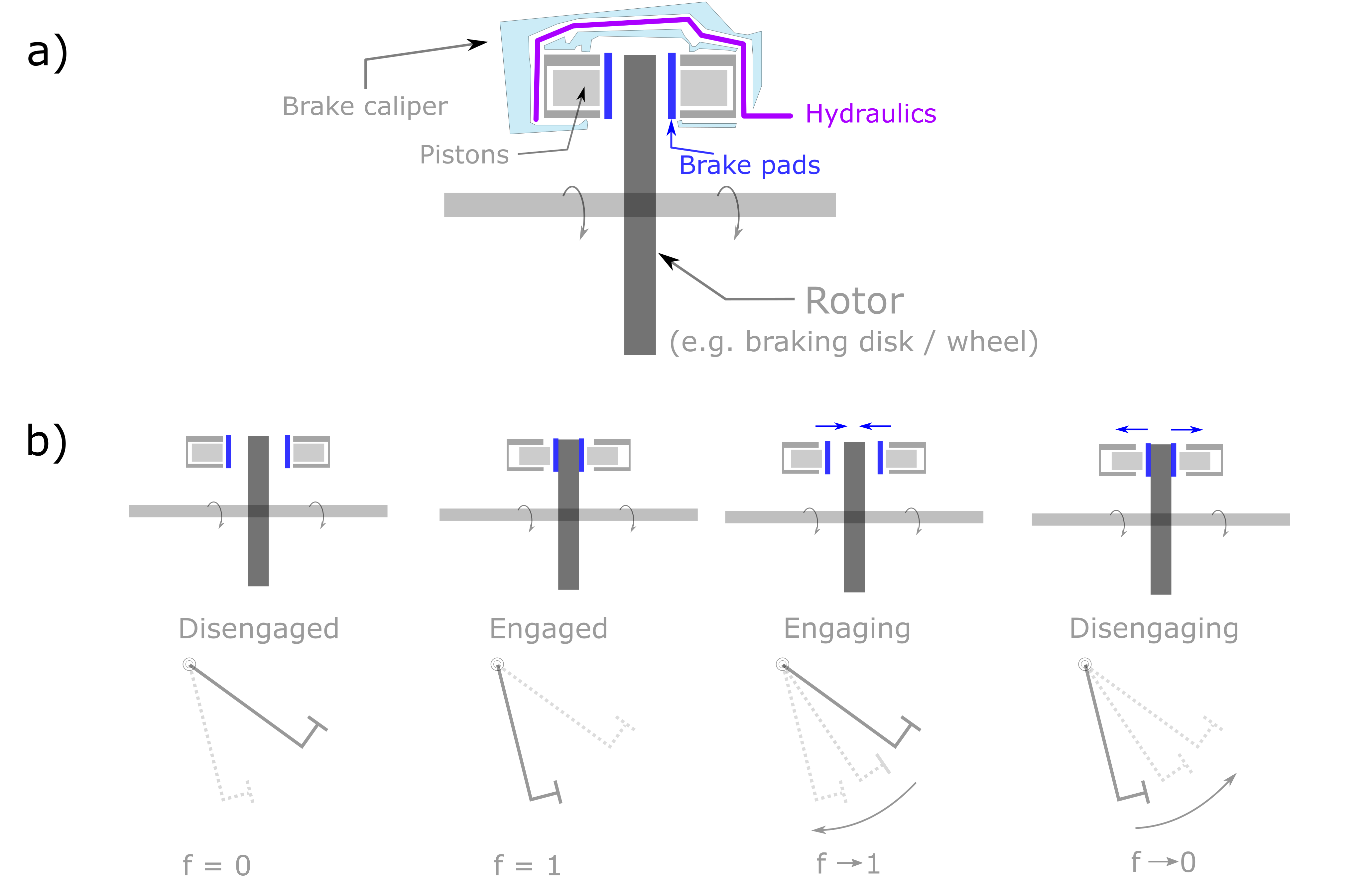
Fig. 19.5 Brake schematic. a) Typical assembly; b) Working mechanism.
A value of \(0\) indicates that the brake is fully disengaged, meaning that the brake pedal is lifted up fully, no braking torque is applied (free rotation). A value of \(1\) refers to a fully engaged brake, meaning that the brake pedal is pressed down fully, full braking (maximum torque transfer) is applied. During the engaging and disengaging process, \(f\) is varying within the range of \([0, 1]\). This parameter simulates how much braking force is applied based on the pedal position.
Note that the brake functions similarly to a DryClutch, but in reverse. While a clutch engages when the pedal is fully released, a brake engages when the pedal is fully pressed. Due to their comparable mechanics, both the Brake and DryClutch share a unified API interface, reflecting their closely related operation.
19.7.1. Governing equations
In AGX, the brake is modelled as a velocity (nonholonomic) constraint attached to a rotational Shaft. The constraint is
where \(\omega\) refers to the angular speed of the shaft, \(\tau\) is the torque transferred via the brake pad, \(\tau_{C}\) is the maximum torque capacity. \(\perp\) is a perpendicularity condition which means that either \(\omega = 0\) and \(-\tau_{C} < \tau < \tau_{C}\), or \(\omega > 0\) and \(\tau = -\tau_{C}\), or \(\omega < 0\) and \(\tau = \tau_{C}\).
This constraint regulates the shaft’s rotation by controlling the magnitude of the torque applied, with two key configurable parameters: the fraction \(f\) and the torque capacity \(\tau_{C}\).
The torque capacity \(\tau_{C}\) is determined by the properties of the brake pads and defines the maximum amount of torque that can be transferred. A higher torque capacity leads to a stronger braking effect, allowing for quicker deceleration as the brake pedal position increases. By adjusting the brake pedal position and torque capacity, the brake model can simulate different braking behaviors, from gradual deceleration to a more immediate stop.
When the lock, i.e. the positional (holonomic) constraint, is activated, the following constraint is enforced
where \(\phi\) refers to the angular position of the shaft. By doing this, the mechnism of the parking brake is modelled. As a result, the shaft remains stationary. In this case, there are no limits on the applied torque.
19.7.2. Parameters
The physical parameters of the Brake are listed below.
Parameter |
Method |
Description |
Default |
\(f\) |
setFraction |
Fraction of the brake pedal postion (or the fraction of the maximum counter torque imposed via the brake pads). Value varying between 0 and 1. |
0 |
\(\tau_{C}\) |
setTorqueCapacity |
The maximum torque that the brake pads can transfer. The unit is N.m |
2000 |
autoLock |
setAutoLock |
Activate the auto lock or not |
True |
engageTimeConstant |
setEngageTimeConstant |
The time required to transition the brake from disengaged to engaged. The unit of the engageTimeConstant is consistent with the time step size defined by the user. The timeConstant varies within the range of \((0, \infty]\), where \(\infty\) indicates that the brake pedal remains in its current position. |
2.5 |
disengageTimeConstant |
setDisengageTimeConstant |
The time required to transition the brake from engaged to disengaged. |
1.0 |
minRelativeSlip |
setMinRelativeSlip |
The threshold to check whether the lock criteria is fulfilled. It is dimensionnless |
1e-5 |
manual |
setManualMode |
Set manual mode or auto mode (See Brake manipulation) |
False |
engage |
setEngage |
Activate engaging (True) or disengaging (False) operation |
False |
The user can customize the above parameters based on desired brake properties, and manuvering and driving preferences.
19.7.3. Build brake
The brake is created and started as:
agxPowerLine::PowerLineRef powerLine = new agxPowerLine::PowerLine();
agxDriveTrain::BrakeRef brake = new agxDriveTrain::Brake();
brake->setTorqueCapacity(1000.0);
brake->setEngageTimeConstant(0.2);
brake->setDisengageTimeConstant(1.0);
brake->setAutoLock(true);
powerLine->add(brake);
Once the brake is built, it can be connected to the other DriveTrain components.
19.7.4. Brake manipulation
The brake can be manipulated with two modes, labelled “manual” and “auto”. In the
manual mode, the user can in great detail control the operation of the brake
using the setFraction() method, see the code snippet below:
class manualBrakeListener : public agxSDK::StepEventListener
{
  public:
    manualBrakeListener(agxDriveTrain::brake* brake) :
    {
    }
    void pre(const agx::TimeStamp& t)
    {
      // Disengaged
      if (t < 1.0) {
        brake->setFraction(0.0);
      }
      // Engaging
      else if (t <= 1.1) {
        brake->setFraction(10 * (t-1));
      }
      // Disengaging
      else if (t <= 3.0) {
        brake->setFraction((3.0-t)/(3-1.1));
      }
    }
In the snippet above, the brake starts to getting engaged quickly at t=1 s and is fully engaged at t=1.1 s, upon which the brake is disengaged relatively slowly, with the brake becoming fully disengaged at t=3.0 s.
In contrast to the manual mode, the setEngage() method can be used to manipulate
the brake automatically.
class autoBrakeListener : public agxSDK::StepEventListener
{
  public:
    autobrakeListener(agxDriveTrain::brake* brake) :
    {
    }
    void pre(const agx::TimeStamp& t)
    {
      // Engaging
      if (t > 3.0 && t <= 5.0)
      {
        brake->setEngage(true);

        // Engage goes from 0 to 1 in 2 seconds.
        brake->setEngageTimeConstant(2.0);
      }
      // Disengaging
      else if (t> 7.0 && t <= 9.0)
      {
        brake->setEngage(false);
        // Disengage goes from 1 to 0 in 1 seconds.
        brake->setDisengageTimeConstant(1.0);
      }
      // Brake on-hold
      else {
        brake->setEngageTimeConstant(math.inf);
        brake->setDisengageTimeConstant(math.inf);
      }
    }
Detailed C++ and python examples with Brake() are available
in tutorials/agxOSG/tutorial_driveTrain_brake.agxPy, tutorials/agxOSG/tutorial_driveTrain_combustionEngine.cpp and
python/tutorials/tutorial_driveTrain_combustinonEngine.agxPy.
19.8. Differential
A differential is a Connector that distributes torque evenly over multiple output shafts in such a way that the angular velocity of the input shaft is the average of the velocities of the output shafts. The differential can be locked, forcing all outputs to rotate at the same speed. There is also a limited slip torque version of the lock, which causes only a limited amount of torque to be transferred between outputs in order to maintain equal velocity of the output shafts.
19.9. Connecting constraints
An Actuator is a powerline component that transfers motion between a powerline unit and a regular AGX constraint. This class will connect a Unit to an ordinary constraint such as a Hinge or Prismatic.
Because a Hinge is a rotational constraint and Prismatic is a translational constraint there are separate sub-classes to the Actuator class: cpp:`agxPowerLine::RotationalActuator and cpp:`agxPowerLine::TranslationalActuator.
So to connect a hinge constraint to an existing drivetrain we use the cpp:`agxPowerLine::RotationalActuator class.
Assuming there exists a wheel body attached to a chassis body using a hinge named hinge, we can drive that wheel with the drive train using the following code.
agxPowerLine::RotationalActuatorRef axle = new agxPowerLine::RotationalActuator(hinge);

// Connect an existing drivetrain (shaft) to the hinge via the RotationalActuator.
shaft->connect(axle);
19.10. Connecting a wire winch to a drivetrain
A agxWire::WireWinchController is a class that can winch in/out wire using a brake and a motor. A WireWinchController is a linear constraint, meaning it operates using a linear force specified in Newton (N). A winch is usually a rotating object with a certain effective radius (depending on how much wire is spooled in). To model a torque driven winch one need to connect a rotational power source such as a motorized Hinge or a Engine.
As the winch is linear and a motor/hinge is rotational, we need to transform rotational work to linear work. This is done using a agxPowerLine::RotationalTranslationalHolonomicConnector.
We also need to connect the connector to a winch and this is done using a agxPowerLine::WireWinchActuator.
We will then end up with a powerline system that looks like:
Hinge---> Shaft ---> RotationalTranslationalHolonomicConnector ---> WireWinchActuator ---> Winch
Below is a sample code snippet that will create this system:
// Assume we have a pointer to a winch object with a routed wire.

// First create a shaft that will transfer rotation between the motorized hinge and the connector below
auto shaft = new agxDriveTrain::Shaft();
auto winch_socket = new agxPowerLine::RotationalTranslationalHolonomicConnector();

// The effective rotation of the "winch" can be specified here
// This will affect the ratio between rotational motion of the hinge and the linear motion of the winch
// A larger radius leads to a higher speed and less force
winch_socket->setShaftRadius( radius );

// Connect the shaft with the winch_socket
shaft->connect( winch_socket );
// Set some small inertia of the shaft. This is the inertia of the rotating drum.
shaft->setInertia( 1e-4 );

// Add the shaft to the powerline
power_line->add( shaft );

// Now create a constraint that will be attached to the shaft rigidbody (1-dimensional)
// First we need to orient the Hinge so that it rotates in the direction of the shaft body
auto frame = new agx.Frame()
frame->setLocalRotate( agx::Quat( agx::Vec3::Z_AXIS(), shaft->getRotationalDimension()->getWorldDirection())  );

// Next we create the hinge
auto winch_hinge = new agx::Hinge( shaft->getRotationalDimension()->getOrReserveBody(), frame );

// We will initially enable the lock of the hinge and disable the motor.
// If we want to winch, we just disable the lock and enable the motor with a target speed.
winch_hinge->getMotor1D()->setEnable( false );
winch_hinge->getMotor1D()->setSpeed( 0 );

// Remember a Lock1D is NOT a brake. It will work as a spring if you violate the target position.
// So either you have to set the position of the lock to avoid a "springback" or, you can use the friction controller
winch_hinge->getLock1D()->setEnable( true );
simulation->add( winch_hinge );

// Finally we create an actuator that will transfer the linear motion from the winch socket to the winch.
auto winch_actuator = new agxPowerLine::WireWinchActuator( winch );
winch_socket->connect( winch_actuator );
power_line->add( winch_actuator );
For a more complete example of this, see the python script data/python/torque_driven_winch.agxPy.