25. Material calibration – bulk materials¶

In AGX Dynamics, AGX Terrain, and Momentum Granular, bulk materials consisting of particles with certain particle parameters can be created. (In agxTerrain, only the dynamic mass of the bulk material consists of particles.) Examples of bulk materials are soils, sands, and gravels, and examples of particle parametes are friction and restitution. A bulk material has certain bulk properties, such as the static angle of repose theta, bulk cohesion c, and friction angle phi, which determine the large scale dynamics of the material. Now, in AGX programs, the particle parameters are set explicitly and yield a particular behavior of the bulk material, i.e. a particular static angle of repose, bulk cohesion, and friction angle will result in one behavior of the bulk material. However, the bulk properties resulting from a certain set of particle parameters are unknown beforehand. Therefore, material calibration tests — the static angle of repose test and the triaxial test — are implemented in AGX Dynamics which determine the bulk properties resulting from a certain set of particle parameters. The static angle of repose test determines the static angle of repose theta, and the triaxial test determines the bulk cohesion c, and the friction angle phi. Thus, the tests offer a mapping between particle parameters and bulk properties.

The point of the tests is to identify the particle parameters that yield the bulk properties of a particular bulk material that the user wants to model (denoted the “desired material”). The process of seeking the particle parameters that yield desired bulk properties is denoted material calibration, and is carried out by using one or both of the tests. If the test with a particular set of particle parameters yield the same bulk property or properties as those of the desired material, the calibration is complete, since then, by using that set of particle parameters, desired bulk properties are yielded. If the result of a test is bulk properties that do not match those of the desired material, the test needs to be repeated with different particle parameters until desired bulk properties are obtained.

This section describes these bulk properties, how the material calibration tests work, and how to carry out the tests and interpret the results.

25.1. Bulk properties¶

As previously noted, bulk materials such as soils, sand, and gravels, have particular bulk properties, for example static angle of repose theta, bulk cohesion c, and friction angle phi. These properties govern the large scale dynamics of the bulk material and can be used to predict for example if a soil will fail under certain conditions, such as if a house is placed on a hill. These properties are independent of simulation implementation and are observed in nature. The static angle of repose is the greatest angle between the side of a static pile and the horizontal plane at which the pile does not slump, see see Fig. 25.1. Typically, a bulk material with high friction has a greater static angle of repose than a bulk material with low friction.

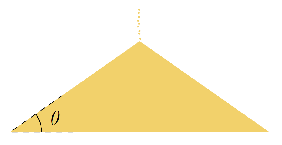
../_images/material_calibration_static_angle_of_repose.png

Fig. 25.1 The static angle of repose theta, illustrated for a pile of sand. The static angle of repose of sand is observed in the lower bulb of an hour glass when the top bulb is empty.¶

For completeness, we also note that there is also the property dynamic angle of repose. For this property, the angle itself is measured essentially as the static angle of repose, but when the material is in motion. This property is for example observed when sand tumbles in a cylindrical mixer. The dynamic angle of repose will not be treated further here.

The shear strength of a material is a function of the friction angle phi (also known and the angle of internal friction), and the bulk cohesion c of the material. These two properties are included in the straight line failure envelope equation, given by

tau = c + tan(phi) * sigma,

where tau is shear stress, and sigma is normal stress, see Fig. 25.2.

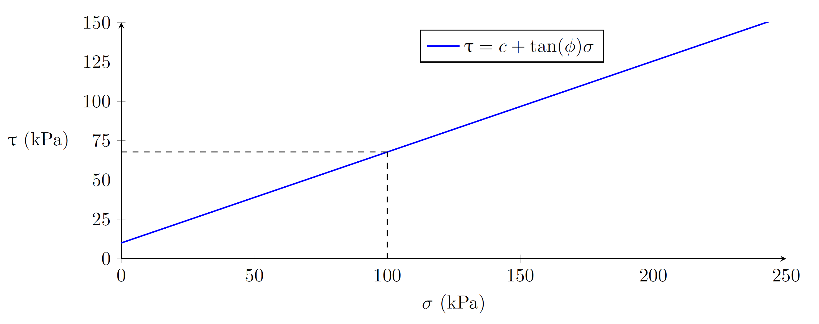
../_images/material_calibration_tau_curve.png

Fig. 25.2 The failure envelope equation, with bulk cohesion c being the intercept, and the tangent of the internal friction phi being the slope. In this particular case, the bulk material has c=10 kPa and phi=30 degrees.¶

The failure envelope equation describes, for a given normal stress, the amount of shear stress a material can withstand without shearing, i.e. failing. Both a higher phi and a higher c implies a greater shear strength. For example, in Fig. 25.2, we note that for this particular material, at a normal stress of 100 kPa, the material shears at a shear stress of 67.7 kPa. At a higher (lower) normal stress, the material shears at a higher (lower) shear stress. That an increased normal stress implies an increased ability to withstand shear stress is exemplified by considering an unopened coffee package under vacuum (coffee, like sand, is a bulk material). In the unopened package, the coffee is in a packed state, with relatively high normal stress, and it is difficult to twist the package, i.e. shear the coffee sample. However, by opening the package (or even by punching a small hole in it with a needle), the normal stress drops significantly, and the package is easily twisted. Shearing is depicted in Fig. 25.3.

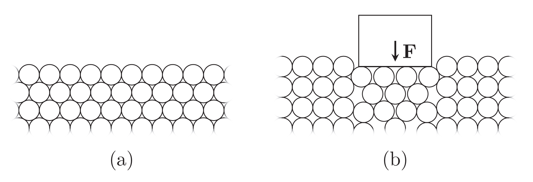
../_images/material_calibration_shearing_of_bulk_material.png

Fig. 25.3 (a) A bulk material, for example sand, represented by spherical particles. The material is in a packed state. (b) A load is applied to the surface of the material. The shear stress is greater than the shear strength so shearing occurs during which particle layers slide over each other: the material fails. Typically, when a bulk material fails, the volume is increased.¶

The friction angle phi is due to contacts and is responsible for an increased shear strength at an increased normal stress: at a higher normal stress, the particles are brought closer, increasing the contacting areas between them and so also the particle-particle frictional forces. The bulk cohesion c is due to attractive cohesive forces and is independent of the normal stress. We note in Fig. 25.2 that an increased c increases the tolerable shear stress with the same amount for all values of the normal stress. Usually, a wet material, for example wet sand, has a higher bulk cohesion than a dry material, as water molecules tend to attract one another—it is easier to build a sand castle with wet or damp sand than with dry sand!

25.2. Selection of particle parameters¶

There is no clear cut strategy in the selection of particle parameters for the material calibration tests. The process is a mix of educated guesses and trial and error. After a completed test, the results give an indication on how to proceed. For example, in the static angle of repose test, if the resulting static angle of repose is lower than the corresponding value of your desired bulk material, a suitable course of action is to repeat the test with a higher friction and/or higher rolling resistance. In the triaxial test, if the resulting bulk cohesion is lower than your desired bulk cohesion, a repeated test with a higher particle cohesion is advisable. One approach, applicable for all tests, is the following: create a (large) number of different particle materials with different particle parameters, place them in a dedicated directory, and then run the test of interest on all of them. This yields several results that you can inspect and compare which gives you a hint on how to proceed.

Now, the particle parameter to bulk properties mappings are not unique. While the bulk properties of a particular bulk material are constant, more than one set of particle parameters can yield one or several of these properties.

25.3. The static angle of repose test¶

The static angle of repose test determines the static angle of repose (described in Bulk properties) and comes in many variants, using a tilted box, fixed funnel, or a hollow cylinder. The test is carried out in real life or with a computer simulation. In this section we describe the test implemented in AGX Dynamics using a hollow cylinder that is lifted, so the full cumbersome name of the test is the “static angle of repose test using the hollow cylinder lifting method”. In Test description we describe how the test works, and in User guide (detailed) we describe in detail how to carry out the test with step by step instructions and how to interpret the results. In User guide (brief) we offer a very short user guide that can be used as a cheat sheet for readers familiar with the test. It is recommended to first read the Test description as this will make the User guide easier to follow and aid in the selection of test settings.

25.3.1. Test description¶

This section chiefly describes the theory and mechanics of the test, and only indirectly describes the workflow for the execution of the test. For a detailed description of the workflow, see User guide (detailed).

25.3.1.1. Setup¶

In the first part of the test setup particle parameters such as friction and rolling resistance are specified. These parameters specify particle-particle interactions and will be applied to the particles that represent the bulk material. Wall parameters — specifying particle-wall interactions — do not be set explicitly as they are automatically calculated from particle parameters. How these are set will be elaborated further. Particle parameters are specified in a particle material file.

In the second part of the test setup simulation settings such as timestep and particle radii are specified in a simulation settings file.

25.3.1.2. The test¶

With particle parameters and simulation settings specified, the test is ready to be executed.

In the 1st phase of the test, “particle emission”, see Fig. 25.4, an emitter (yellow cylinder) moves slowly upwards and emits particles. The particles land on a static base (violet cylinder). The particles are surrounded by an initially static tall hollow cylinder (light blue), preventing them from falling of the base. Below the base, there is a static particle sink (blue cylinder of large radius), .

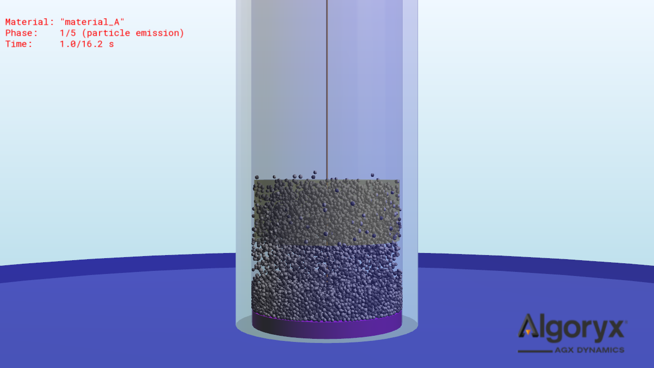
../_images/material_calibration_saor_t_one_dot_zero.png

Fig. 25.4 The test in the 1st phase: “particle emission”. The selected particle material file is material_A.json.¶

In the 2nd phase, “particle sample relaxation”, see Fig. 25.5, the particle sample is allowed to rest for a short duration, allowing particle velocities to drop to essentially zero.

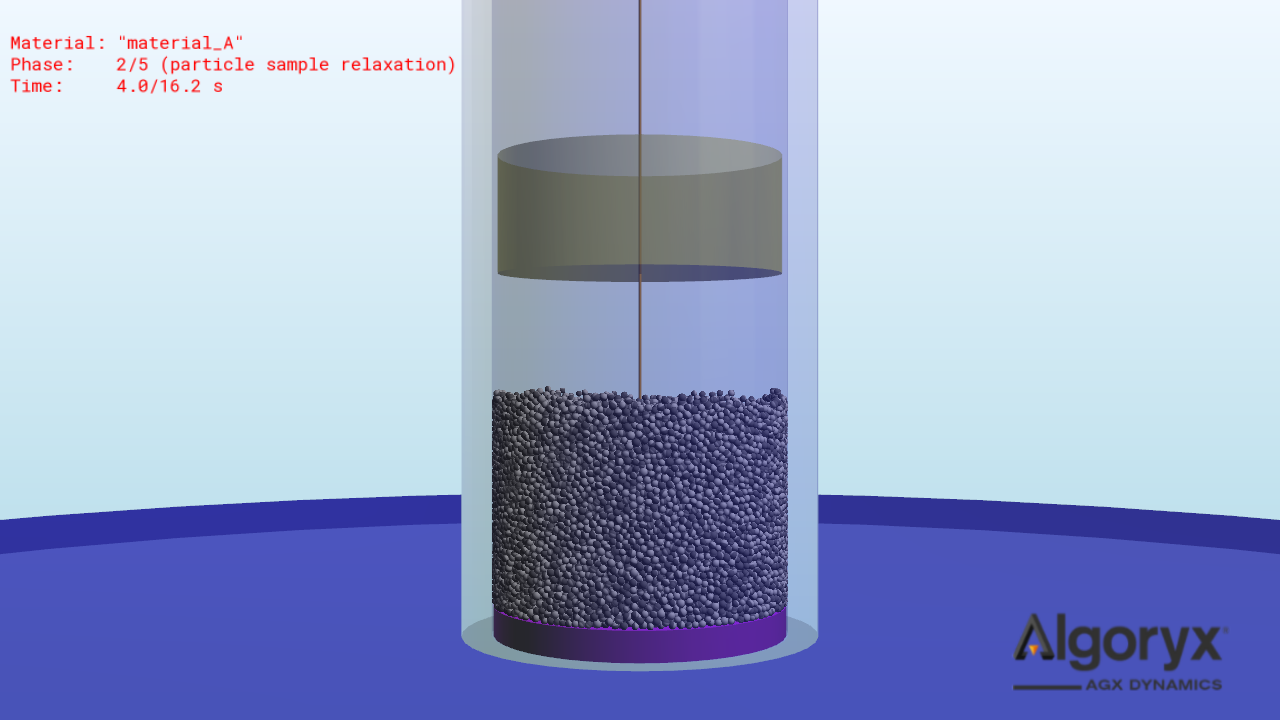
../_images/material_calibration_saor_t_four_dot_zero.png

Fig. 25.5 The test in the 2st phase: “particle sample relaxation”.¶

In the 3rd phase, “cylinder lifting”, see Fig. 25.6, the hollow cylinder is slowly lifted, allowing particles to fall off the base and towards the sink where they are removed. By removing particles that fall of the base, the computational time is decreased. Now, the static angle of repose is independent of the height of the particle pile. Therefore, the top surface of the base can be considered to be a slice of the pile. Thus, the base-particle interactions are set to be the same as the particle-particle interactions. However, we would like the hollow cylinder to interact as little as possible with the particle sample, so we set zero friction in the hollow cylinder-particles interactions.

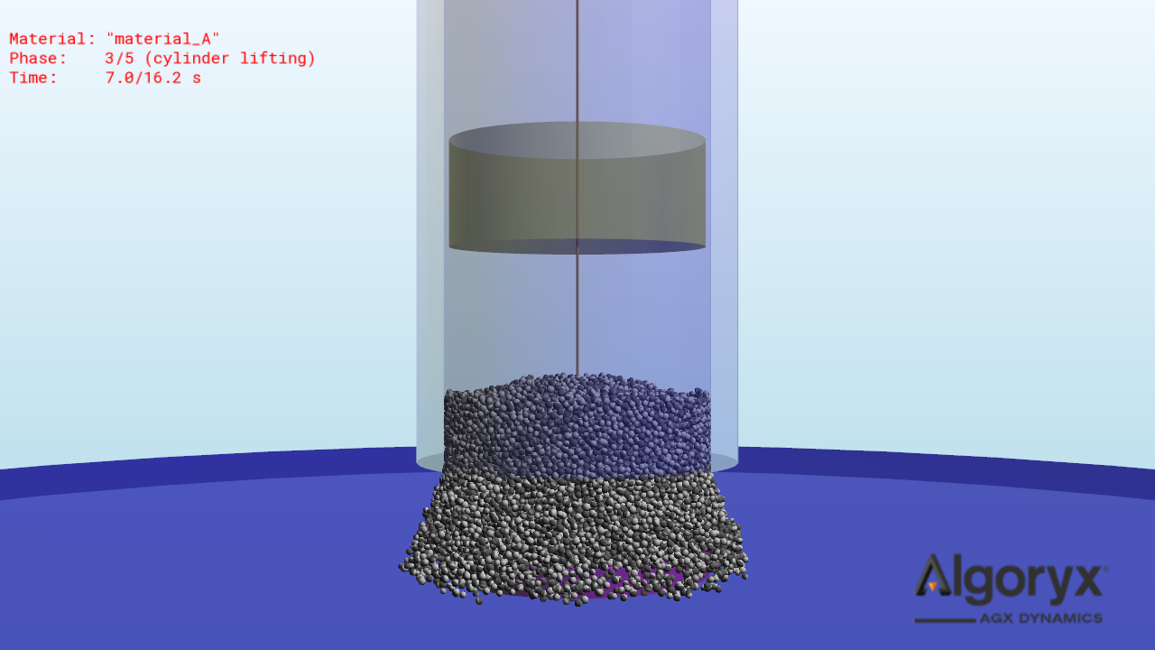
../_images/material_calibration_saor_t_seven_dot_zero.png

Fig. 25.6 The test in the 3rd phase: “cylinder lifting”.¶

In the 4th phase, “particle pile relaxation”, Fig. 25.7, the particle sample is allowed to rest for a short duration, again allowing particle velocities to drop to essentially zero. At the end of this phase, a static granular pile has formed with some static angle of repose.

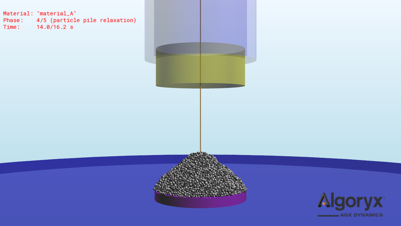
../_images/material_calibration_saor_t_fourteen_dot_zero.png

Fig. 25.7 The test in the 4th phase: “particle pile relaxation”.¶

25.3.1.3. The analysis¶

In the 5th phase, “particle pile analysis”, the particle pile is analyzed by an algorithm by which angle of repose results are obtained. The surface of the base is parallel to the \(xy\)-plane, \(z\) is the vertical axis, \(r=\sqrt{x^2+y^2}\) is the polar radial coordinate, and \(\psi=\mathrm{atan}(y/x), x>0\) is the azimuthal angle.

For the analysis, \(n_{\mathrm{slices}}\) slices are introduced such that slice \(i=1,2,...,n_{\mathrm{slices}}\) is the plane \(\psi_i=(i-1)(360^\circ/n_{\mathrm{slices}})\). Each slice has \(n_{\mathrm{cells}}\) associated cylindrical cells of radius \(R_{\mathrm{cell}}\) and infinite height with axes parallel to the \(z\)-axis and in the plane of the slice such that cell \(j=1,2,...,n_{\mathrm{cells}}\) is centered at \(r_j=jR_b/(n_{\mathrm{slices}}+1)\), where \(R_b\) is the radius of the base. \(R_{\mathrm{cell}}\) is larger than the largest particle radius of the particle system. These elements are illustrated in Fig. 25.8.

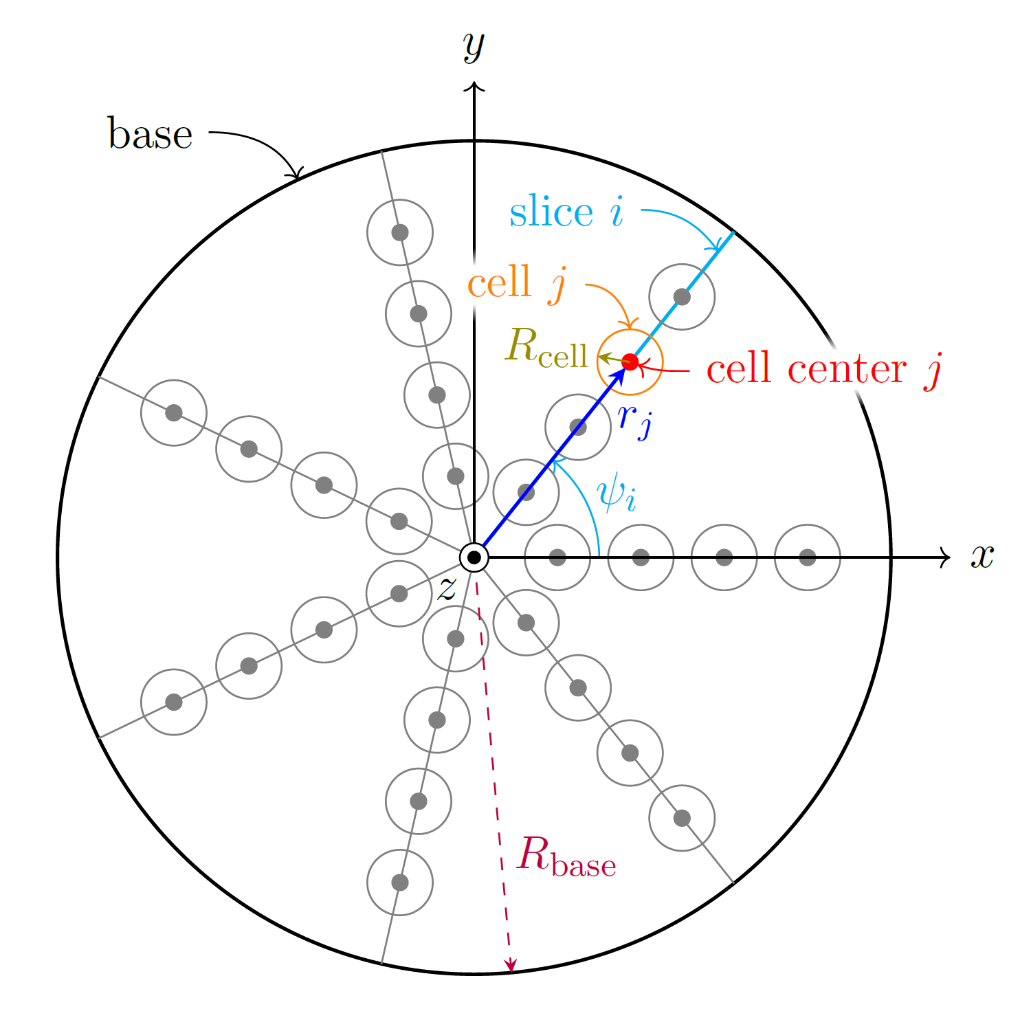
../_images/material_calibration_saor_analysis_elements.png

Fig. 25.8 A top view (looking down the \(z\)-axis) of the test, with emphasis on the analysis elements. We recall that the base is the cylinder of radius \(R_{\mathrm{base}}\) upon which the particles rest. Slice \(i\), making an angle \(\psi_i\) with the \(x\)-axis, is highlighted. Also highlighted is cell \(j\) of slice \(i\) and its associated quantities: \(r_j\) is the distance from the origin to the cell center, and \(R_{\mathrm{cell}}\) is the radius of the cell. In this figure, there are \(7\) slices, and \(4\) cells, yielding a total of \(7\times 4=28\) cells.¶

For each cell, all particles within the cell are considered by the algorithm (for cell \(j\) of slice \(i\), the particles considered are within the region indicated by the orange circle in Fig. 25.8), and the particle with the largest \(z\)-coordinate is selected for that cell and its \(r\)- and \(z\)-coordinates are stored. This particle is also colored, giving a three dimensional presentation of the analysis algorithm, see Fig. 25.9.

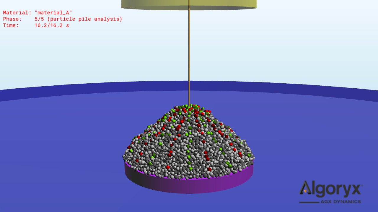
../_images/material_calibration_saor_t_sixteen_dot_two_alt.png

Fig. 25.9 The test in the 5th phase: “particle pile analysis”. For a particular slice, the associated particles with the largest \(z\)-coordinates are colored by a single color, red or green. In this case, the pile is divided into 20 slices, and each slice is divided into 15 cells. Thus, we have 20 strings of colored particles, with 15 particles in each string.¶

For each slice, a linear least-squares regression is applied to the associated sets of the \(z\)- and \(r\)-coordinates of the particles with the largest \(z\)-coordinates, yielding a straight line with a slope such that the arctangent of the slope approximates the static angle of repose for that slice. Thus, for \(n_{\mathrm{slices}}\) slices, we have \(n_{\mathrm{slices}}\) approximations of the static angle of repose. From these \(n_{\mathrm{slices}}\) approximations, we obtain the average static angle of repose, the standard deviation of the average, the minimum angle, and the maximum angle. The test and analysis is complete.

25.3.2. User guide (brief)¶

The static angle of repose test is performed by executing the following steps:

Find the static angle of repose theta of your desired bulk material
Make sure that required python modules are installed (see static_angle_of_repose_test/requirements.txt)
Create your particle material(s) (see e.g. particle_soil/json/sand_1.json)
Set up the simulation settings file (see static_angle_of_repose_test/SimConfDefault.py)
Open an AGX terminal at /static_angle_of_repose_test/ and run the static angle of repose test (runStaticAngleOfReposeTest.py)
Inspect the test result(s) (stored in static_angle_of_repose_test/results/). If the static angle of repose theta matches the value of the desired bulk material, the material calibration is complete. If not, rerun the static angle of repose test with different particle parameters until desired static angle of repose is yielded.

25.3.3. User guide (detailed)¶

25.3.3.1. Find the static angle of repose `theta` of your desired bulk material¶

The static angle of repose theta of a particular material can be found by consulting a table of soil or granular materials, if the material is not too uncommon. If tables are inaccessible or do not exist, physical experiments on the real material need to be carried out to measure the property. If such experiments are infeasible, the property needs to be judiciously estimated.

25.3.3.2. Locate the static angle of repose test¶

Your AGX Dynamics installation path should be on the form C:/.../AGX-<version>. Then, the static angle of repose test is located at AGX-<version>/data/python/material_calibration/particle_soil/static_angle_of_repose_test.

25.3.3.3. Install python modules¶

The test is written in python and the modules required for the static angle of repose test are listed in static_angle_of_repose_test/requirements.txt. Make sure that they are installed for the python version specified to be used with AGX Dynamics. To install the modules, use e.g. python -m pip install -r requirements.txt.

25.3.3.4. Create your particle material(s)¶

Browse to /particle_soil/json/. This is the directory in which particle materials are stored and should be created. The particle sample in the static angle of repose test will have particle parameters of a file from this directory or a subdirectory of it, say /particle_soil/json/my_materials/. More specifically, these parameters set particle-particle interactions. (Particle-wall interactions do not need to be specified.) For convenience, copy one of the existing files, for example sand_1.json, rename the file to, say, material_A.json and enter desired particle parameters and save the file. An example is shown in Code snippet 1.

{
    "soilName" : "MATERIAL_A",
    "ParticleProperties" : {
      "particleCohesiveOverlapRatio" : 0.025,
      "particleCohesion" : 0,
      "particleDamping" : 4.5,
      "particleFriction" : 0.45,
      "particleRestitution" : 0.1,
      "particleRollingResistance" : 0.25,
      "particleSpecificDensity" : 2700,
      "particleYoungsModulus" : 1e9
    }
}

Code Snippet 1 - material_A.json

Notes on how to select particle parameters are given in Selection of particle parameters.

The material in Code snippet 1 is used for the simulation demonstrated in Test description: the test.

25.3.3.5. Set up the simulation settings file¶

The simulation settings file with default settings is static_angle_of_repose_test/SimConfDefault.py. In Code snippet 2 an abbreviated version of this file is given.

class SimConf():
    def __init__(self, particleSpecificationPath=defaultSpecificationPath, particleSpecification=""):

        ### Simulation parameters ###
        self.timeStep = 1/1000
        self.numPPGSRestingIterations = 500
        self.agxOnly = False
        ...

        ### Particle material ###
        self.particleRadius = 0.015
        self.particleRadiusMin = 0.9 * self.particleRadius
        self.particleRadiusMax = 1.1 * self.particleRadius
        self.particleWeight = 0.4
        self.particleWeightMin = 0.3
        self.particleWeightMax = 0.3
        ...

        ### Static angle of repose test parameters ###
        self.baseRadius = 0.6
        self.numSlices = 20
        self.numCells = 15
        ...

Code Snippet 2 - An abbreviated version of SimConfDefault.json

In this file simulation settings such as time step, particle radii, etc. are specified. If you desire to alter these simulation settings, it is recommended to save them in a new file, say static_angle_of_repose_test/SimConfMySettings.py. Usually, the default values can be used for most settings. The settings of most interest are shown in Code snippet 2.

The time step (self.timeStep) and the number of iterations for the iterative solver (self.numPPGSRestingIterations) have an impact on the static angle of repose. Both a larger time step and a smaller number of iterations usually result in a smaller static angle of repose. It is recommended, if possible, to use the same time step and number of iterations in the test as in the simulation in which you desire to use your bulk material. Computational time is roughly linearly proportional to the simulation frequency (the inverse of the time step) and linearly proportional to the number of iterations. self.agxOnly sets graphics on/off. With self.agxOnly = True only the simulations are carried out, and with self.agxOnly = False simulations are carried out and windows are opened in which graphics are rendered. self.agxOnly is important to consider if you run the tests on a computer using a remote connection. With self.agxOnly = False, access to open windows may be denied which results in a crash. If you use a remote connection, self.agxOnly = True is recommended.

Up to three different particle radii can be specified (self.particleRadius, self.particleRadiusMin, and self.particleRadiusMax). self.particleRadius is the basis for the calculation of the cohesive overlap. The particles carry weights such that the particles of radius self.particleRadius will constitute self.particleWeight / (self.particleWeight + self.particleWeightMin + self.particleWeightMax) of the total mass of the particle sample, and similarly for the particles of radii self.particleRadiusMin and self.particleRadiusMax. With the settings in Code snippet 2, the particles of radius self.particleRadius will constitute 0.4 / (0.4 + 0.3 + 0.3) = 0.4 of the total mass, i.e. 40%. The particle radii have an effect on the static angle of repose, so it is recommended to use the same particle radii in the test as in your simulation.

The number of particles to emit is calculated from the particle radii and the radius of the base (self.baseRadius). A larger self.baseRadius to self.particleRadius ratio will increase the number of particles emitted. More particles imply a more refined slope of the granular pile, and a greater precision in the calculation of the static angle of repose. With the assumption that the particle radii are approximately equal, and the particle weights are approximately equal, the following ratio is recommended: self.baseRadius / self.particleRadius > 30. Computational time is roughly linearly proportional to the number of particles, so increasing the mentioned ratio can drastically increase the computational time. For example, by doubling the ratio, the number of particles is increase by a factor of roughly eight. self.numSlices specifies the number of slices to divide the granular slice into (i.e. the number of individual angles of repose to calculate), and self.numCells specifies the number of cells associated with each slice. Both an larger number of slices and a larger number of cells increase the number of points for the calculation, increasing accuracy in the angles of repose calculations. However, too many slices and cells is unwanted since it runs the risk of overlapping cells such that a particular particle can be the particle with the highest \(z\)-coordinate in two or more cells.

The settings in Code snippet 2 are used for the simulation demonstrated in Test description: the test.

25.3.3.6. Run the static angle of repose test¶

The static angle of repose test should be started with /static_angle_of_repose_test/ as the current working directory. For example, start an AGX terminal and browse to /static_angle_of_repose_test/. To start the static angle of repose test, run runStaticAngleOfReposeTest.py with appropriate arguments. Two examples are

python runStaticAngleOfReposeTest.py SimConfDefault.py material_A.json

python runStaticAngleOfReposeTest.py SimConfMySettings.py my_materials

The first example executes the static angle of repose test for json/material_A.json with simulation settings specified in SimConfDefault.py. The second example executes the static angle of repose test for all particle materials in the directory json/my_materials/ with simulation settings specified in SimConfMySettings.py. A full description on how to specify arguments is found by consulting runStaticAngleOfReposeTest.py. As you hit enter, the static angle of repose test with be executed.

25.3.3.7. Inspect the test results¶

When the test or tests have completed, bar graphs (one per material) are stored as pdfs in static_angle_of_repose_test/fig/ , and result files (one per material) are stored as json files in static_angle_of_repose_test/results/. We begin by considering the result file from a test with material_A.json, see Code snippet 3.

{
     "Description": {
          "date": "2022-10-16 19:21:24",
          "test": "static_angle_of_repose_test",
          "particleSpecification": "material_A"
     },
     "ResultsFromIndividualAnglesOfRepose": {
          "averageAngleOfRepose": 37.536869070161906,
          "standardDeviation": 0.8914828660521458,
          "minAngleOfRepose": 35.89691538629683,
          "maxAngleOfRepose": 39.4879976298608
     },
     "IndividualAnglesOfRepose": [
          39.4879976298608,
          37.89848285992389,
          38.58629975167365,
          38.59317117760724,
          37.86961668429997,
          37.1151311577757,
          36.796149118478375,
          37.78694513210245,
          38.57604638098495,
          36.59148912637279,
          36.88952461601244,
          37.17808882132403,
          37.46446064702305,
          36.13803741623653,
          36.67545555864243,
          37.976255819948385,
          37.111137010605276,
          38.14838087881512,
          35.89691538629683,
          37.957796229254164
     ],
     "ParticleProperties": {
          "particleRadiusMin": 0.0135,
          "particleRadiusMedium": 0.015,
          "particleRadiusMax": 0.0165,
          "particleWeightMin": 0.3,
          "particleWeightMedium": 0.4,
          "particleWeightMax": 0.3,
          "particleCohesiveOverlapRatio": 0.025,
          "particleCohesion": 0.0,
          "particleDamping": 4.5,
          "particleFriction": 0.45,
          "particleRestitution": 0.1,
          "particleTwistingResistanceCoefficient": 0.01,
          "particleRollingResistance": 0.25,
          "particleSpecificDensity": 2700.0,
          "particleYoungsModulus": 1000000000.0
     },
     "BaseProperties": {
          "baseCohesiveOverlapRatio": 0.025,
          "baseCylCohesion": 0.0,
          "baseCohesion": 0.0,
          "baseDamping": 4.5,
          "baseFriction": 0.45,
          "baseRestitution": 0.1,
          "baseTwistingResistanceCoefficient": 0.01,
          "baseRollingResistance": 0.25,
          "baseSpecificDensity": 2700.0,
          "baseYoungsModulus": 1000000000.0
     },
     "HollowCylProperties": {
          "hollowCylCohesiveOverlapRatio": 0.025,
          "hollowCylCohesion": 0.0,
          "hollowCylDamping": 4.5,
          "hollowCylFriction": 0.0,
          "hollowCylRestitution": 0.0,
          "hollowCylRollingResistance": 0.0,
          "hollowCylTwistingResistanceCoefficient": 0.01,
          "hollowCylSpecificDensity": 2700.0,
          "hollowCylYoungsModulus": 1000000000.0
     },
     "SimulationParameters": {
          "timeStep": 0.001,
          "numPPGSRestingIterations": 500,
          "useParallelPGS": true,
          "useGranularWarmStarting": true,
          "use32bitGranularBodySolver": true,
          "gravitationalAcceleration": -9.81
     }
     "TestParameters": {
          "baseRadius": 0.6,
          "numberOfSlices": 20,
          "numberOfCells": 15,
          "cellRadius": 0.02475,
          "hollowCylSpeed": 0.625
          "emissionDuration": 3,
          "postEmissionRelaxDuration": 2,
          "postGranularPileFormationRelaxDuration": 4,
     }
}

Code Snippet 3 - The result file for material_A.json: result_static_angle_of_repose_test_material_A.json

All essential settings of the test and key results are summarized in the result file (Code snippet 3).

The key results are located under "ResultsFromIndividualAnglesOfRepose". "averageAngleOfRepose" is the average static angle of repose (which is the arithmetic mean of the individual static angles of repose in "IndividualAnglesOfRepose"), "standardDeviation" is the standard deviation of "averageAngleOfRepose", "minAngleOfRepose" is the minimum static angle of repose (the smallest value in "IndividualAnglesOfRepose"), and "maxAngleOfRepose" is the largest static angle of repose (the largest value in "IndividualAnglesOfRepose"). We see that the central result of the test, for one standard deviation, is the following average angle of repose:

\[\theta = 37.54 \pm 0.89 ^\circ.\]

Under "ParticleProperties" the particle parameters specified by "particleSpecification" and used in the test that describe particle-particle interactions are given. Also, the particle radii used and their weights are reported. The objects "ParticleProperties" and "ResultsFromIndividualAnglesOfRepose" together constitute the sought mapping between particle parameters and bulk properties: the particle material with particle parameters given by "ParticleProperties" will yield a bulk material with the static angle of repose "averageAngleOfRepose".

Under "BaseProperties" particle-base interactions are given, and under "HollowCylProperties" particle-hollow cylinder interactions are specified.

We now inspect the bar graph of the test, see Fig. 25.10.

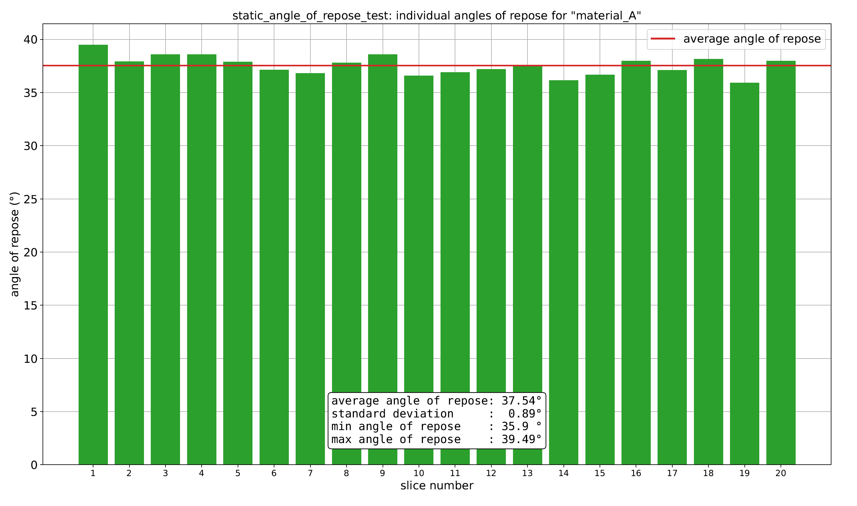
../_images/material_calibration_saor_bar_graph.png

Fig. 25.10 The bar graph for material_A.json: bar_graph_static_angle_of_repose_test_my_gravel.pdf. Individual angles of repose for each slice are visualized, with quantities calculated from them summarized in a box.¶

The bar graph provides a convenient overview of the results of the test.

25.3.3.8. Evaluate test results¶

With the test results checked out, it’s time to evaluate them. If averageAngleOfRepose agress sufficiently well with the corresponding value of your desired bulk material, the material calibration is complete with respect to the static angle of repose. You then enter the used particle parameters in the static angle of repose test in the applicable program (AGX Dynamics, agxTerrain, or Momentum Granular). This yields desired bulk properties with respect to the static angle of repose. If averageAngleOfRepose does not agree sufficiently well with the value of your bulk material, the test needs to be repeated with different particle parameters until a desired averageAngleOfRepose is obtained, see Selection of particle parameters.

25.4. The triaxial test¶

The triaxial test determines the bulk cohesion c and friction angle phi (described in Bulk properties). The test is carried out in real life or with a computer simulation. In this section we describe the test implemented in AGX Dynamics. In the test, a particle sample is confined in a container, and is subjected to stresses. We consider the container to be a cubic box surrounded by 6 walls, with the \(z\)-axis pointing upwards, and the bottom wall parallel to the \(xy\)-plane. In the horizontal directions (the \(x\)- and \(y\)-directions), the sample is subjected to a constant specified stress by moving the vertical walls in appropriate directions. This stress is denoted the consolidation stress. If the consolidation stress drops below the specified stress, the vertical walls move toward the center of the sample, and if it exceeds the specified stress, the vertical walls move away from the center. This keeps the consolidation stress constant. In the vertical direction (\(z\)-direction), the horizontal walls move toward the center with constant speed and a variable force is applied to these walls such that this constant speed is maintained. As the horizontal walls move toward the center, the vertical pressure increases such that it exceeds the consolidation stress. This difference in stresses in the vertical and horizontal directions introduces a shearing stress in the particle sample. The vertical stress increases up until the point where the sample fails by shearing. When the soil shears, the sample expands and the vertical stress drops. The consolidation stress and the vertical stress are stored regularly during the test. The test is then repeated several times for different consolidation stresses. By analyzing the stress data, bulk properties can be obtained.

In Test description we describe how the test works, and in User guide (detailed) we describe in detail how to carry out the test with step by step instructions and how to interpret the results. In User guide (brief) we offer a very brief user guide that can be used as a cheat sheet for readers familiar with the test. It is strongly recommended to first read the Test description as this will illuminate the steps in the User guide, particularly the interpretation of the results.

25.4.1. Test description¶

25.4.1.1. Setup¶

In the first part of the test setup particle parameters such as friction and rolling resistance are specified. These parameters specify particle-particle interactions and will be applied to the particles that represent the bulk material. Particle parameters are specified in a particle material file. Wall parameters — specifying particle-wall interactions — are specified in a wall material file.

25.4.1.2. Creation of an initial simulant¶

With particle parameters and simulation settings configured, the triaxial test and associated simulations can now be executed. This first part in this process is the creation of a so called initial simulant, using the model CreateSimulant.agxPy, see Fig. 25.11.

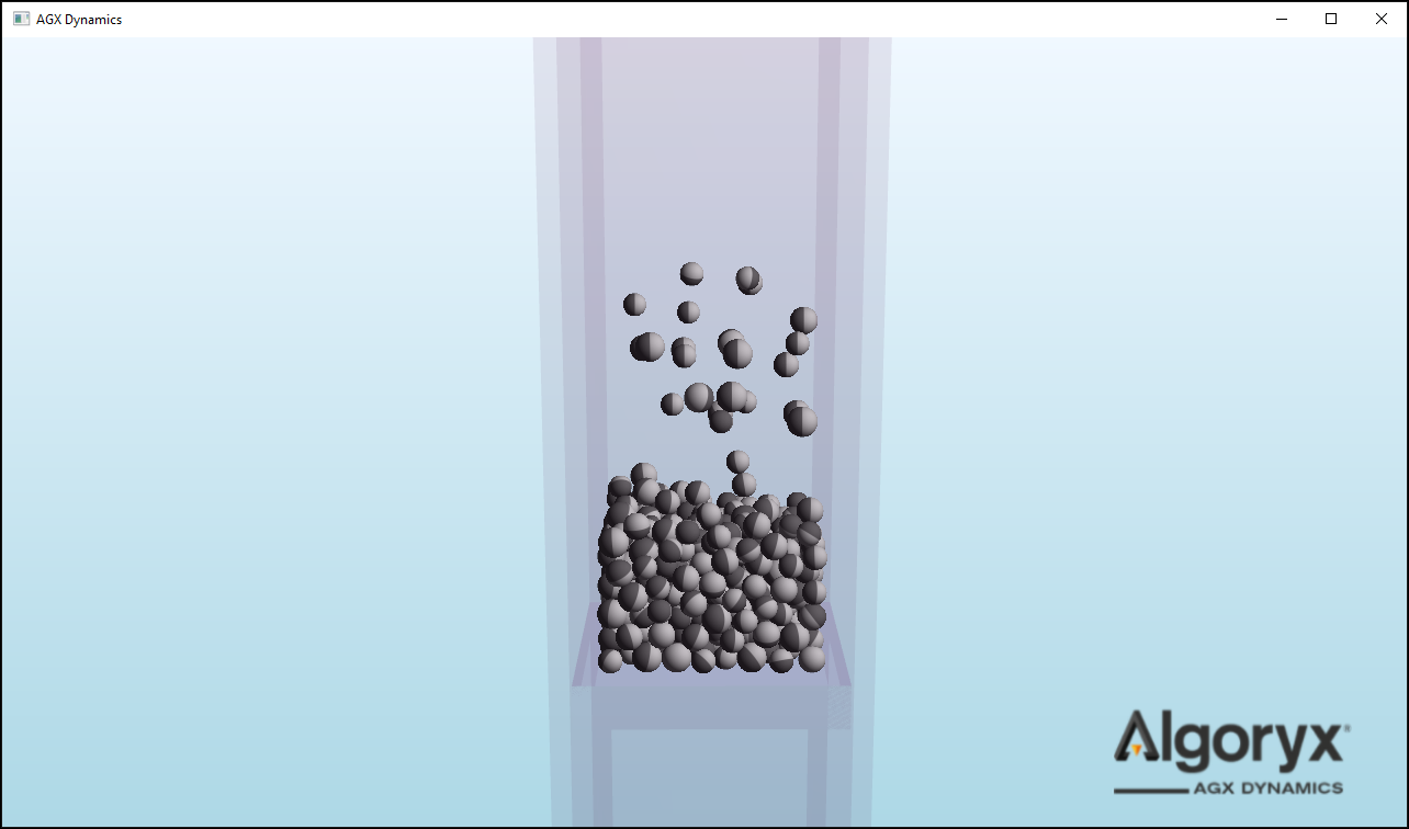
../_images/material_calibration_triaxial_create_initial_simulant.png

Fig. 25.11 Creation of an initial simulant.¶

During the creation of the initial simulant, particles a spawned in a rectangular container in a loose state until a rectangular sample has formed. Then, the sample is saved.

25.4.1.3. Consolidation of initial simulant¶

Next, the saved initial simulant from the previous step is loaded into a rectangular box using consolidation.agxPy, see Fig. 25.12.

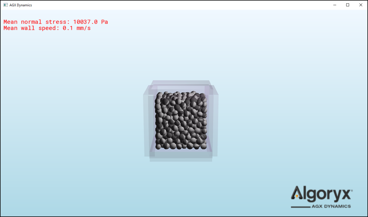
../_images/material_calibration_triaxial_consolidation.png

Fig. 25.12 Consolidation of the initial simulant.¶

During the consolidation the walls are moved such that the specified consolidation stress, which is 10 kPa in Fig. 25.12, is reached. If the stress drops below 10 kPa, the walls are driven towards the center of the sample. If the stress exceeds 10 kPa, the walls are driven away from the center. When the relative error between the actual measured stress and the specified stress goes below a small number, the soil sample is saved.

25.4.1.4. Triaxial test of the consolidated sample¶

Now the preparatory simulations are complete. Next, the saved consolidated sample from the previous step is loaded into the triaxial test using triaxialTest.agxPy, see Fig. 25.13.

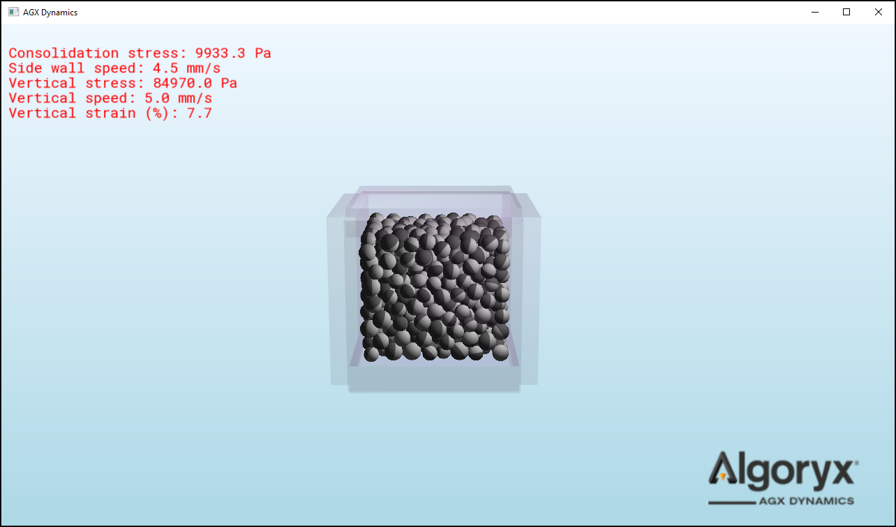
../_images/material_calibration_triaxial_test.png

Fig. 25.13 The triaxial test.¶

During the triaxial test, the vertical walls move such that the horizontal stresses are maintained at the consolidation stress (10kPa in Fig. 25.13). The horizontal walls move towards the center in the vertical direction with constant speed, increasing the vertical pressure. We note that at a vertical strain (compression) of 7.7%, the vertical stress is 84.97 kPa. The pressures are continuously stored in a data file. By comparing Fig. 25.12 and Fig. 25.13, we note that the sample has been compressed in the vertical direction and expanded in the horizontal directions in Fig. 25.13.

25.4.1.5. Repetition of triaxial test¶

The consolidation and triaxial test are then repeated a number of times, say, 10 times, for different consolidation pressures. After these repetitions the test is complete.

25.4.1.6. Identifications of bulk properties¶

We recall that for each run, the consolidation stress and vertical stress are stored at regular short intervals. Also, the particular stresses at which the soil fails need to be identified in order to determine bulk properties. An automatically generated plot of the stresses as a function of vertical displacement from a triaxial test is shown in Fig. 25.14.

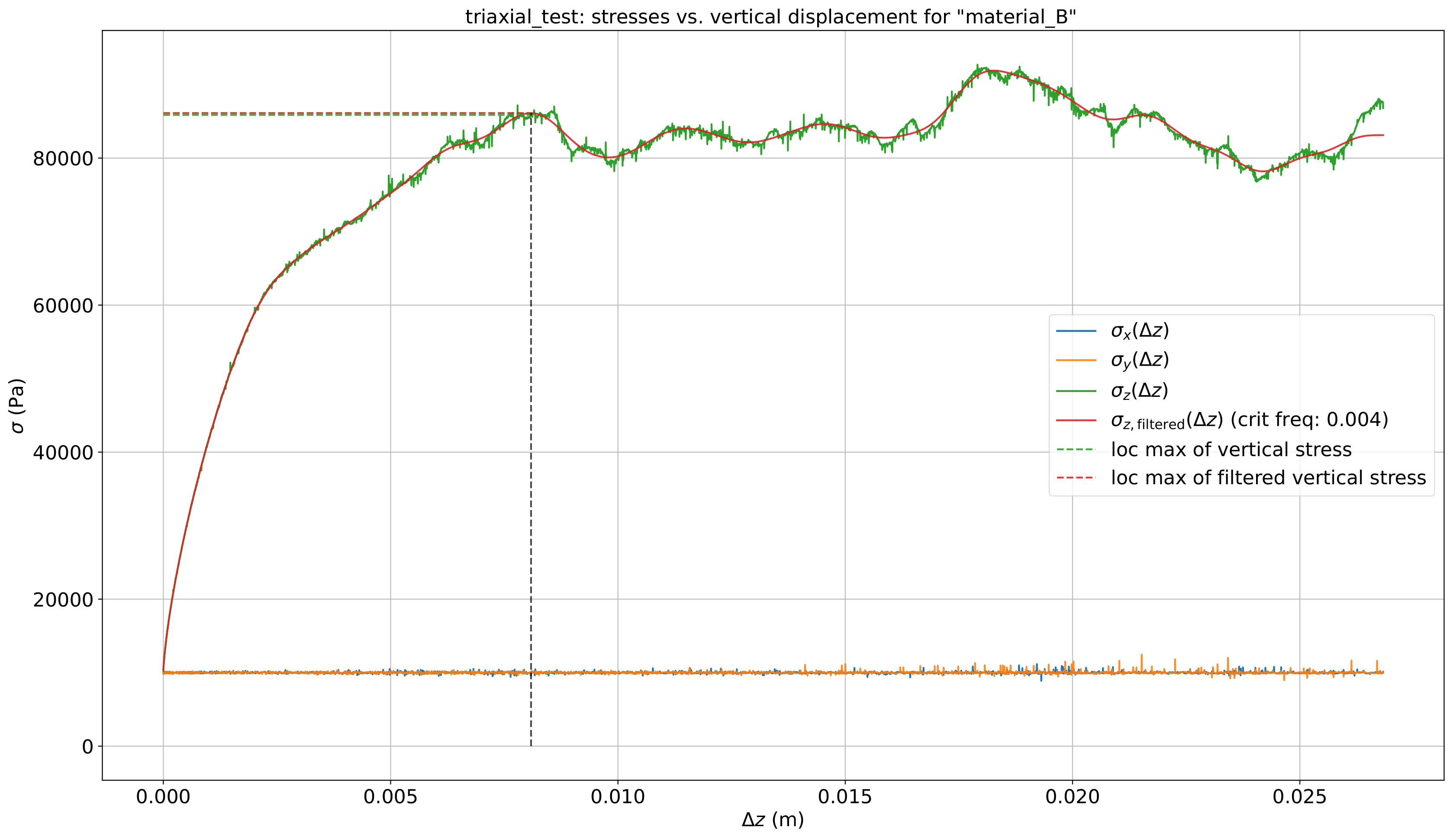
../_images/material_calibration_triaxial_stress_triaxial_test_material_B_10000Pa.png

Fig. 25.14 Stresses (\(\sigma\), sigma) as functions of the vertical displacment (\(\Delta z\), Delta z) for a triaxial test with a consolidation stress of 10 kPa.¶

The plot in Fig. 25.14 shows the evolution of the stresses (y-axis) as a function of the vertical displacement of the walls (x-axis). The plot is from the triaxial test in Fig. 25.13. We note that the measured horizontal stresses, sigma_x and sigma_y, representing the consolidation stress, lie close to the specified consolidation stress of 10 kPa, as desired. As the sample is more and more compressed in the vertical direction, i.e. as the vertical displacement increases, we note that the vertical stress sigma_z increases. As described earlier, when the soil fails and shears, it expands, resulting in a drop in vertical pressure. An algorithm using a filtered version of the vertical stress seeks to identify this point of failure, which usually is the first local maximum of a filtered version of sigma_z. This identification is indicated by the dashed lines in Fig. 25.14. With a visual inspection, we note that this indeed seems to be where the vertical stress drops.

Now, the key results from the simulations are stored in a .json file. The following is an abbreviated example (result_triaxial_test_material_B.json).

{
        "Description": {
            "date": "2022-09-23 11:10:12",
            "test": "triaxial_test",
            "particleSpecification": "material_B"
        },
        "BulkPropertiesFromBulkData": {
            "c": 4.737650504718438,
            "phi": 46.09,
            "standardError_c": 0.4726372802858118,
            "standardError_phi": 0.46488510277406264
        },
        "BulkData": {
            "consolidationStress": [
                5069.832186961724,
                10036.720190218033,
                15334.126180643405,
                ...
            ],
            "verticalStress": [
                50377.87891396498,
                85868.52312832276,
                117089.52718754749,
                ...
            ]
        },
        "ParticleProperties": {
            "particleRadiusMin": 0.0135,
            ...
        },
        "SimulationParameters": {
            "timeStep": 0.0003333333333333333,
            ...
        },
        "FilterParameters": {
            "filterOrder": 4,
            ...
        }
}

Code Snippet 4 - result_triaxial_test_material_B.json (abbreviated, as indicated by the ....)

Consider Code snippet 4. In the first run (with a specified consolidation stress of 5000 Pa), the algorithm has identified the point where the soils fails by shearing to be at the consolidation stress of 5069.8 Pa, and the vertical stress of 50378 Pa. Similarly, in the second run (with a specified consolidation stress of 10000 Pa), the consolidation and vertical stresses at failure are 10037 Pa and 85869 Pa, respectively (this is the failure that is indicated by the dashed lines in Fig. 25.14), and so on. The data in BulkData is used to calculate the bulk cohesion c and friction angle phi, and the standard errors standardError_phi (associated with phi) and standardError_c (associated with c). Let us see how by inspecting Fig. 25.15.

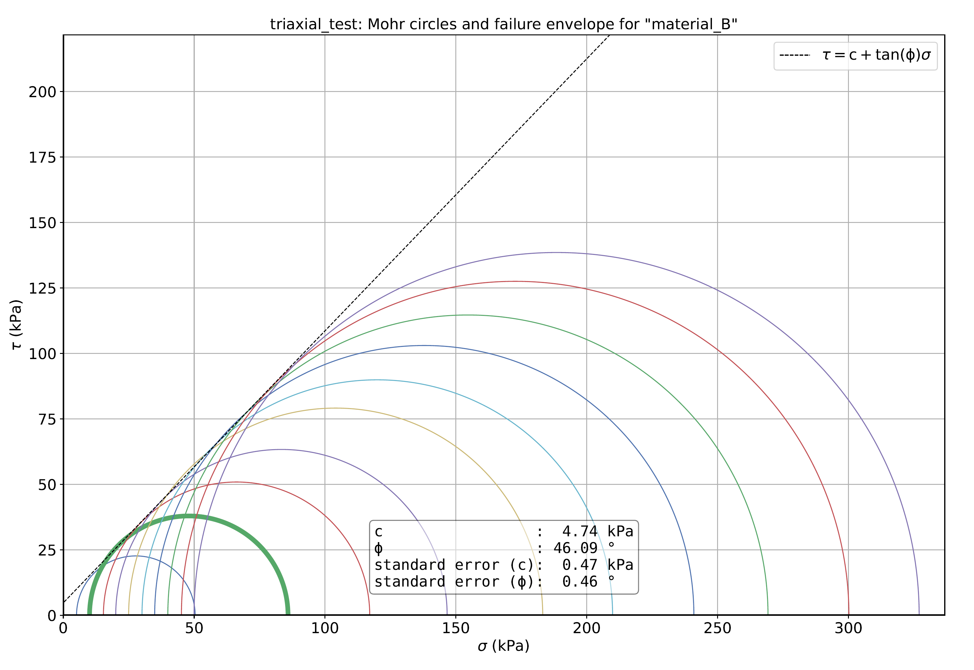
../_images/material_calibration_triaxial_bulk_properties_triaxial_test_material_B_green_highlighted.png

Fig. 25.15 Mohr circles and Mohr-Coulomb failure envelope created from the stresses at soil failure of the triaxial tests.¶

The plot in Fig. 25.15 is constructed from the stresses in bulkData in result_triaxial_test_material_B.json (see Code snippet 4). We note that there are 10 semi-circles known as Mohr circles, each one corresponding to a triaxial test with a particular specified consolidation pressure. For result_triaxial_test_material_B.json, the specified consolidation pressures are [5000, 10000, ..., 45000, 50000] Pa, hence 10 semi-circles. Each semi-circle is constructed such that the right-most x-coordinate of it is the vertical stress, and the left-most x-coordinate is the consolidation stress (these coordinates lie on the x-axis). The green semi-circle in Fig. 25.15, highlighted with a thick line, corresponds to the test with the specified consolidation stress 10 kPa, see Fig. 25.14. By inspecting Fig. 25.15, we see that the right-most coordinate of the thick green semi-circle is around 85 kPa, which is the recorded vertical stress of 85869 Pa at failure (see result_triaxial_test_material_B.json). Moreover, again by inspection of Fig. 25.15, we see that the left-most coordinate of the thick green semi-circle is around 10 kPa, which is the recorded consolidation stress of 10037 Pa at failure. If the algorithm fails to identify the point of soil failure, appropriate measures need to be taken (see User guide (detailed): Inspect the unvalidated test results).

The final step in order to obtain bulk properties is to construct a straight line that is tangent to all these semi-circles. This straight line is known as the Mohr-Coulomb failure envelope, and is on the form

tau = c + sigma * tan(phi),

where tau is shear stress, and sigma is normal stress. The failure envelope is fitted to be tangent to the semi-circles by linear least squares regression. The linear regression also yields standards errors: std_err_slope is associated with phi, and std_err_intercept is associated with c. In Fig. 25.15, the failure envelope is the dashed straight line. This particular failure envelope has c=4.74 kPa, and phi=46.09 degrees, as noted in the plot. These are the bulk properties yielded from the triaxial test. The triaxial test process is complete.

25.4.2. User guide (brief)¶

The triaxial test is performed by executing the following steps:

Find the bulk cohesion c and friction angle phi of your desired bulk material
Make sure that required python modules are installed (see triaxial_test/requirements.txt)
Create your particle material(s) (see e.g. particle_soil/json/sand_1.json)
Set up the simulation settings file (see triaxial_test/SimConfDefault.py)
Open an AGX terminal at /triaxial_test/ and run the triaxial test (runTriaxialTest.py)
Inspect the unvalidated test result(s) (stored in triaxial_test/results/)
Inspect the failure envelope (stored in triaxial_test/fig/)
Validate the stress plots (stored in triaxial_test/fig/)
1. If needed, adjust the simulation settings file and use triaxial_test/replotAll.py
2. If needed, adjust vertical failure stress values in the test result(s) and use triaxial_test/replotFailureEnvelope.py
Inspect the validated test result(s). If the bulk cohesion c and the friction angle phi match the values of the desired bulk material, the material calibration is complete. If not, rerun the triaxial test with different particle parameters until desired bulk properties are yielded.

25.4.3. User guide (detailed)¶

In the following we provide detailed step by step instructions on how to execute the triaixal test.

25.4.3.1. Find the bulk properties `c` and `phi` of your desired bulk material¶

The bulk properties c and phi of a particular material can be found by consulting a table of soil or granular materials, if the material is not too uncommon. If tables are inaccessible or do not exist, physical experiments on the real material need to be carried out to measure properties. If such experiments are infeasible, properties need to be judiciously estimated.

25.4.3.2. Locate the triaxial test¶

Your AGX Dynamics installation path should be on the form C:/.../AGX-<version>. Then, the triaxial test is located at AGX-<version>/data/python/material_calibration/particle_soil/triaxial_test.

25.4.3.3. Install python modules¶

The test in written in python and the required modules are listed in triaxial_test/requirements.txt. Make sure that they are installed for the python version specified to be used with AGX Dynamics. To install the modules, use e.g. python -m pip install -r requirements.txt.

25.4.3.4. Create your particle material(s)¶

Browse to /particle_soil/json/. This is the directory in which particle materials are stored and should be created. The soil sample in the triaxial test will have particle parameters of a file from this directory or a subdirectory of it, say /particle_soil/json/my_materials/. More specifically, these parameters specify particle-particle interactions. For convenience, copy one of the existing files, for example sand_1.json, rename the file to, say, material_B.json and enter desired particle parameters and save the file. An example is shown in Code snippet 5.

{
    "soilName" : "MATERIAL_B",
    "ParticleProperties" : {
      "particleCohesiveOverlapRatio" : 0.025,
      "particleCohesion" : 7500,
      "particleDamping" : 4.5,
      "particleFriction" : 0.35,
      "particleRestitution" : 0.1,
      "particleRollingResistance" : 0.35,
      "particleSpecificDensity" : 2200,
      "particleYoungsModulus" : 1e9
    }
}

Code Snippet 5 - material_B.json

You can create more than one material and run triaxial tests on more than one material in one go. Also, you can place several materials in a new directory in /particle_soil/json/, say /particle_soil/json/my_materials/, and perform triaxial tests on all materials in that folder.

Wall parameters — specifying particle-wall interactions — are specified in triaxial_wall.json (see /particle_soil/json/). Default wall parameters are specified in this file. (These values can be adjusted if needed.)

25.4.3.5. Set up the simulation settings file¶

The simulation settings file with default settings is triaxial_test/SimConfDefault.py. In Code snippet 6 an abbreviated version of this file is given.

class SimConf():
    def __init__(self, particleSpecificationPath=defaultSpecificationPath, particleSpecification="")

        ### Simulation parameters ###
        self.timeStep = 1/2000
        self.numPPGSRestingIterations = 400
        self.agxOnly = False
        ...

        ### Particle material ###
        self.particleRadius = 0.015
        self.particleRadiusMin = 0.9 * self.particleRadius
        self.particleRadiusMax = 1.1 * self.particleRadius
        self.particleWeight = 0.4
        self.particleWeightMin = 0.3
        self.particleWeightMax = 0.3
        ...

        ### Triaxial test parameters ###
        self.wallSideLength = 0.25
        ...

        ### Signal filter parameters ###
        self.filterOrder = 4
        ...

Code Snippet 6 - SimConfDefault.json

In this file simulation settings such as time step, particle radii, etc. are specified. If you desire to alter these simulation settings, it is recommended to save them in a new file, say triaxial_test/SimConfMySettings.py. Usually, the default values can be used for most settings. The settings of most interest are shown in Code snippet 6.

The time step (self.timeStep) and the number of iterations for the iterative solver (self.numPPGSRestingIterations) have an impact on the bulk properties. It is recommended, if possible, to use the same time step and number of iterations in the test as in the simulation in which you desire to use your bulk material. Computational time is roughly linearly proportional to the simulation frequency (the inverse of the time step) and linearly proportional to the number of iterations. For an explanation of self.agxOnly, see SimfConfDefaut (static angle of repose test).

For the setting of particle radii, see SimfConfDefaut (static angle of repose test).

Various parameters of the test can be specified such as length of walls (self.wallSideLength), wall speeds, etc. are specified. Default values are recommended for ### Triaxial test parameters ###. See SimConfDefault.py for additional information.

For the identification of failure points a filtered signal of the vertical stress is used. The parameters of the filter are specified here. self.filterOrder specifies the order of the filter. Default values are recommended for ### Signal filter parameters ###. See SimConfDefault.py for additional information.

25.4.3.6. Run the triaxial test¶

Start an AGX terminal and browse to /triaxial_test/. This is the directory from which the triaxial test should be run. To start the triaxial test, run runTriaxialTest.py with appropriate arguments. Two examples are

python runTriaxialTest.py SimConfDefault.py material_B.json

python runTriaxialTest.py SimConfMySettings.py my_materials

The first example executes the triaxial test for material_B.json with simulation settings specified in SimConfDefault.py. The second example executes the triaxial test for all particle materials in the directory json/my_materials with simulation settings specified in SimConfMySettings.py. A full description on how to specify arguments is found by consulting runTriaxialTest.py. As you hit enter, the triaxial test with associated simulations will be executed.

25.4.3.7. Inspect the unvalidated test result(s)¶

When the triaxial test has completed, plots describing strain, stress, etc. are stored in triaxial_test/fig/ and key results are stored in triaxial_test/results/. For example, if your particle parameter file is material_B.json, then plots are stored in triaxial_test/fig/material_B/, and a key result file are stored in triaxial_test/results/result_triaxial_test_material_B.json. We begin by considering the result file. In Code snippet 7 an example result file is shown.

{
      "Description": {
          "date": "2022-09-23 11:10:12",
          "test": "triaxial_test",
          "particleSpecification": "material_B"
      },
      "BulkPropertiesFromBulkData": {
          "c": 4.737650504718438,
          "phi": 46.09,
          "standardError_c": 0.46488510277406264,
          "standardError_phi": 0.4726372802858118,
      },
      "BulkData": {
          "consolidationStress": [
                5069.832186961724,
                10036.720190218033,
                15334.126180643405,
                20042.03025732538,
                24971.475941893936,
                30081.725345084255,
                34924.68195807154,
                39947.85331379516,
                45142.31398754626,
                49976.82805899259
          ],
          "verticalStress": [
                50377.87891396498,
                85868.52312832276,
                117089.52718754749,
                146661.62243417173,
                183183.91905994146,
                209881.79120832373,
                240935.25233170495,
                269258.88806409494,
                300170.4442784592,
                327011.1903817603
          ]
      },
      "ParticleProperties": {
          "particleRadiusMin": 0.0135,
          "particleRadiusMedium": 0.015,
          "particleRadiusMax": 0.0165,
          "particleWeightMin": 0.3,
          "particleWeightMedium": 0.4,
          "particleWeightMax": 0.3,
          "particleCohesiveOverlapRatio": 0.025,
          "particleCohesion": 7500.0,
          "particleDamping": 4.5,
          "particleFriction": 0.35,
          "particleRestitution": 0.1,
          "particleRollingResistance": 0.35,
          "particleSpecificDensity": 2200.0,
          "particleYoungsModulus": 1000000000.0
      },
      "SimulationParameters": {
          "timeStep": 0.0003333333333333333,
          "numberOfPPGSRestingIterations": 500,
          "consolidationSpeed": 0.0025,
          "horizontalSpeed": 0.1,
          "verticalSpeed": 0.005,
          "horizontalAcceleration": 10,
          "verticalAcceleration": 0.01
      },
      "FilterParameters": {
          "filterOrder": 4,
          "criticalFrequency": 0.004,
          "minVertStressToConsStressRatio": 1.25
      }
}

Code Snippet 7 - results_triaxial_test_material_B.json

All essential settings of the triaxial test and key results are summarized in the result file (Code snippet 7). The date of the test and the name of the particle material are given under Description. The key results are located under bulkPropertiesFromBulkData. c is the bulk cohesion (in kPa), and phi is the friction angle (in degrees) associated with the particle material material_B.json. standardError_phi is the standard error associated with phi, and standardError_c is the standard error associated with c. The stresses at which soil failure occur are given in BulkData. For example, in the first test, soil failure occurs at the condolisation stress of 5069.8 Pa and the vertical stress of 50378 Pa. The data in BulkData is used to calculate the results in bulkPropertiesFromBulkData, as the name of that object suggests. The particle parameters used for the triaxial test, i.e. the particle parameters that are associated with the bulk properties in bulkPropertiesFromBulkData, are given in particleProperties. The simulating settings are located under simulationParameters, and the filter parameters used are given in filterParameters.

25.4.3.8. Inspect the Mohr-Coulomb failure envelope¶

Next we inspect the Mohr-Coulomb failure envelope, see Fig. 25.15.

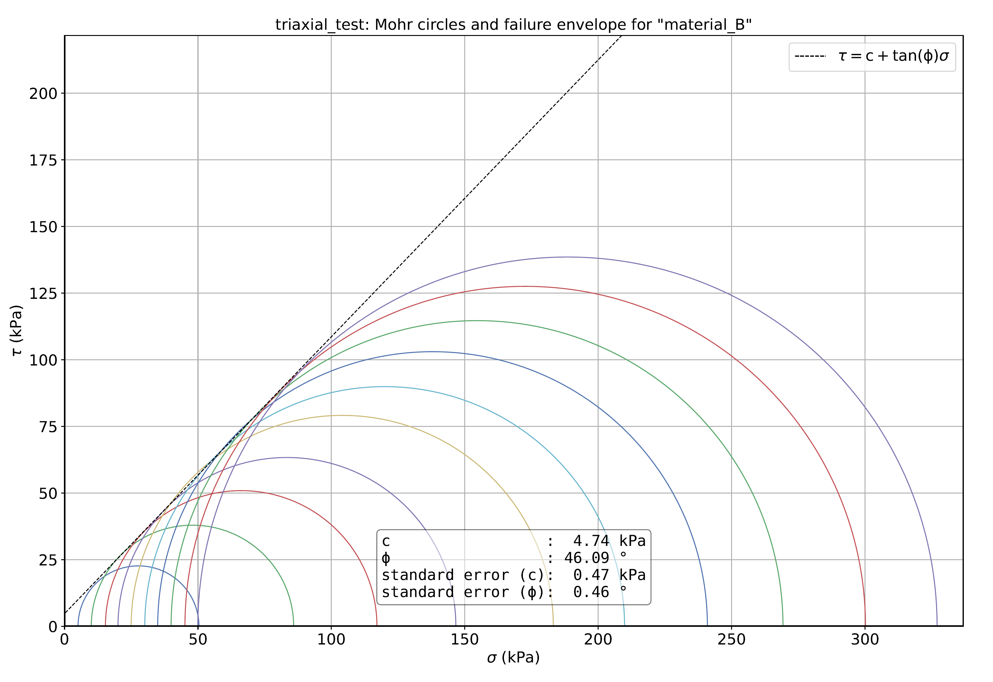
../_images/material_calibration_triaxial_bulk_properties_triaxial_test_material_B.png

Fig. 25.16 The Mohr Coulomb failure envelope of fig/bulk_properties_triaxial_test_material_B.pdf.¶

If all or most semi-circles are just tangent to the failure envelope (the straight dashed line), this is an indication that test results are reliable. We note in Fig. 25.15 that this is the case. If one or more circles clearly deviate from this behaviour, this is an indication that the failure point identification algorithm has failed for the tests associated with those circles. (We note that the straight line is not entirely tangent to the semi-circle with right-most x-coordinate between 150 and 200 kPa, but the deviation is minor.) In any case, it is best to validate the stress plots, as described in the next step.

25.4.3.9. Validate the stress plots¶

To validate the results described in the previous step, we study the stress plots. In Fig. 25.17, we show fig/material_B/triaxial_stress_triaxialTest_material_B_10000Pa.pdf, with the ending of the file name indicating that the consolidation stress is specified to 10 kPa.

Fig. 25.17 Stresses (\(\sigma\), sigma) as functions of the vertical displacment (\(\Delta z\), Delta z) for a triaxial test with a consolidation stress of 10 kPa.¶

We check that the algorithm has correctly identified the point at which the soil fails, i.e. where the vertical stress drops. We see that the algorithm seems to have identified the correct point.

Now, since the consolidation stress is essentially constant throughout the test, as desired, the algorithm only needs to identify the correct vertical stress. This means that if the failure point reported by the algorithm is to the right (perhaps even far to the right) of the actual failure point (as determined by visual inspection), but the reported failure point has essentially the same vertical stress as the actual failure point, we can consider the algorithm to have correctly identified the failure point, since then the reported vertical stress of failure is essentially identical to the actual vertical stress of failure (and the reported consolidation stress of failure is essentially identical to the actual consolidation stress of failure, since the consolidation stress is essentially constant throughout the test). This is a subtle but important argument, and the takeaway is to check if the reported failure point agrees with the actual failure point with respect to only the y-axis, and not both the x- and y-axis.

All stress plots (one for each specified consolidation stress) should be inspected to see if the reported failure points agree decently with the actual failure points. However, sometimes it is difficult to visually identify the failure point even with keen observing due to the sensitivity of the test, noise and the complicated behaviour of the vertical stress curve. At any rate, if the reported failure points agree with the actual failure points, the test results are validated and you can move to the next step.

If however, one or more reported points differ substantially from the actual failure points, there are two appropriate actions, denoted A and B, that can be taken:

A. Reconfigure the simulation settings

Reconfigure the filter by changing filter parameters in the simulation settings file, see In Code snippet 6. Then use runReplotAll.py to only update the plots with the new filter parameters and recompute the results file. This is a fast computation and does not rerun the triaxial test. To carry out this action, do as follows. Let’s say that you ran the triaxial tests with
python runTriaxialTest.py SimConfMySettings_A.py material_B.json
Then you can simply configure new filter parameters in, say, SimConfMySettings_B.py, and run
python runReplotAll.py SimConfMySettings_B.py material_B.json
This updates all plots and the test results file according to the settings in SimConfMySettings_B.py. If this yields satisfactory identification points, the test results are validated and you can move the the next step.

For more details, consult runReplotAll.py

B. Manually adjust vertical stresses

If different filter settings do not improve the identification of failure points satisfactorily, you need to manually specify vertical stresses in the result file. The procedure is as follows. Consider the abbreviated result file in Code snippet 8.
{
     "Description": {
          "date": "2022-09-23 11:10:12",
      "test": "triaxial_test",
          "particleSpecification": "material_B"
     },
     "BulkPropertiesFromBulkData": {
          "c": 4.737650504718438,
          "phi": 46.09,
          "standardError_phi": 0.4726372802858118,
          "standardError_c": 0.46488510277406264
     },
     "BulkData": {
          "consolidationStress": [
               5069.832186961724,
               10036.720190218033,
               15334.126180643405,
               ...
          ],
          "verticalStress": [
               50377.87891396498,
               85868.52312832276,
               117089.52718754749,
               ...
          ]
     },
     ...
}
Code Snippet 8 - result_triaxial_test_material_B.json with an incorrect vertical stress for the 3rd test.

If the reported failue point is incorrect in, say, the 3rd test, i.e. the vertical stress of 117089.5 Pa is incorrect, we need to adjust that value. Let’s say that the actual vertical stress is 130000 Pa, as determined by visual inspection. Then, we replace the original value with the new value, such that the file in Code snippet 8 is obtained.
{
     "Description": {
          "date": "2022-09-23 11:10:12",
          "particleSpecification": "material_B"
     },
     "BulkPropertiesFromBulkData": {
          "c": 4.737650504718438,
          "phi": 46.09,
          "standardError_phi": 0.4726372802858118,
          "standardError_c": 0.46488510277406264
     },
     "BulkData": {
          "consolidationStress": [
               5069.832186961724,
               10036.720190218033,
               15334.126180643405,
               ...
          ],
          "verticalStress": [
               50377.87891396498,
               85868.52312832276,
               130000,
               ...
          ]
     },
     ...
  }
Code Snippet 8 - triaxial_result_material_B.json with the incorrect vertical stress for the 3rd test replaced with the correct value.

We then save the file (without chaning its name) and use RunReplotFailureEnvelope.py. This will update the plot of the failure envelope, and consequently also the results in bulkPropertiesFromBulkData since the results in than object is obtained from the failure envelope. To carry out this action, do as follows. Let’s say that you ran the triaxial test with
python runTriaxialTest.py SimConfMySettings_A.py material_B.json
and perhaps also
python runReplotAll.py SimConfMySettings_B.py material_B.json
as described in A. (If you did or did not use runReplotAll.py does not matter.) Then, to update the plot of the failure envelope and the results in bulkPropertiesFromBulkData, run
python runReplotFailureEnvelope.py SimConfMySettings_C.py material_B.json
where SimConfMySettings_C.py is either SimConfMySettings_A.py or SimConfMySettings_B.py (it does not matter). As the manoeuver of replacing vertical stress values is independent of the filter algorithm and the triaxial test itself, this will, with respect to plots in fig/material_B/, only update the failure envelope plot and not the other plots.

After this manual adjustments and the execution of runReplotFailureEnvelope.py, the test results are validated and you can move to the next step.

For more details, consult runReplotFailureEnvelope.py.

25.4.3.10. Inspect the validated test result(s)¶

When the test results have been validated, it’s time to compare them against the values of your desired bulk material. If c and phi agree with the values of the desired bulk material, the material calibration is complete with respect to c and phi. You then enter the used particle parameters in the triaxial test in AGX Dynamics, agxTerrain, or Momentum Granular. This yields desired bulk properties of the bulk material with respect to c and phi. If c and phi do not match the values of the desired bulk material, the test needs to be repeated with different particle parameters until desired bulk properties are obtained.