9. Creating stable simulations¶

Creating stable simulations is an art. It requires the juggling of a large set of parameters and attributes. This chapter will try to summarize a few of the most important things to keep in mind.

9.1. Masses¶

Depending on the selected solver (iterative or direct), the mass ratio between interacting bodies can become a problem. The default solver setting in AGX is a hybrid scheme where all constraints including ordinary constraints and contacts are handled with the direct solver, except for the friction of contacts, which are handled by the iterative solver. The hybrid solver is able to handle large mass ratios in stacking and constrained systems.

For the iterative solver (when specifying constraints or contacts to be solved iteratively) it is very important to keep the masses in the system in the same range of order of magnitude. For example a rigid body of mass 0.1 which interacts (collides with, is constrained to) with one that weighs 100 might cause instabilities due to large mass ratios. In general (but especially when using the iterative solver), try to keep mass ratios as low as possible, or at least for interacting objects. Having objects with mass 1gram in the same simulation as objects with 100E3Kg is ok, as long as they don’t interact with each other.

9.2. Damping¶

In AGX Dynamics, contacts and constraints have an amount of damping, just like in the real world, due to friction, elasticity and other effects. Apart from modeling damped systems, damping has also an effect on the numerics and thus on the stability of the simulation.

Damping for contacts can either be set through the material properties;

Material::getBulkMaterial()::setDamping( )

or more preferably through the use of explicit ContactMaterial.

Damping is also important when using constraints. Assume for example that you have created a cylinder which is attached to the world with a hinge. If the hinge does not have a target speed-, lock- or friction controller enabled, nothing will stop the cylinder from rotating once it starts (unless the body itself has velocity damping enabled).

In real life, there is always friction in bearings, air-resistance etc. that will add “damping” to a system. This is something to keep in mind when you want to create stable simulations.

The damping coefficient set in AGX Dynamics for contacts and constraints is given in the unit of time, and differs from the typically used viscous damping coefficient. Use the functions in agxUtil::convert in order to convert from the viscous damping coefficient to AGX’ damping coefficient. See 12.1.1 for more information.

A separate topic is the concept of body velocity damping, which is sometimes applied in simulations for numerical reasons, or to mimic aerodynamic or hydrodynamic effects. In AGX Dynamics, body velocity damping is disabled by default, since aerodynamic and hydrodynamic effects are better modeled with the dedicated library in AGX (see chapter 22).

However, velocity damping of a rigid body can be done the following way:

RigidBody::setVelocityDamping(double)
RigidBody::setLinearVelocityDamping(double)
RigidBody::setAngularVelocityDamping(double)

Valid values are between 0 and any real value, 0 is no damping (default). The velocity damping is a viscous damping.

9.3. Time step¶

The time step or dt used when stepping a simulation forward is very important. To get stable simulations one should use consistent time steps, that is, always stepping the simulation forward with same dt. Stepping a simulation with different dt might introduce energy and cause instabilities. Always strive to use the shortest possible dt, the shorter, the more stable simulations. Collision detection relies on that all collisions can be caught during one step. So if a geometry is moving fast relative to its size, or collides with a relative small geometry, penetration, or tunneling effects can occur. This will result in large penetrations or even missed collisions. Large penetrations will create large forces that will try to restore the penetrated geometry outwards.

Changing the time step is done via the agxSDK::Simulation object:

#include <agxSDK/Simulation.h>

// Create a Simulation which holds the DynamicsSystem and Space.
agxSDK::SimulationRef sim = new agxSDK::Simulation;

// Set the time step to 0.01s (100hz)
sim->setTimeStep( 1.0/100.0 );

Consider the simple case of two objects colliding below.

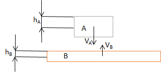
Fig. 9.1 Two objects moving towards each other.¶

In Fig. 9.1 we have two objects A and B that are moving towards each other and will at some point collide. Collision detection is done after moving the objects, so they will overlap to a certain degree. The object’s relative velocity \(V_{rel}=V_A - V_B\) will determine the total impact speed at collision. The distance these two objects will cover during one time step is \(S_{dt} = V_{rel} * \Delta t\). We need to make sure that the time step is small enough so the following expression is fulfilled:

\begin{equation} \Delta t : [S_{dt} << min(h_A, h_B)] \end{equation}

I.e. \(\Delta t\) is chosen small enough so that the distance the two objects cover during one time step is much smaller than the half extent of the smallest object.

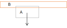
Fig. 9.2 \(\Delta t\) is too large. Object A will pass through object B.¶

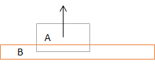
Fig. 9.3 \(\Delta t\) is small enough. Object A will bounce out of object B in a correct manner.¶

9.4. Size of objects¶

As described in the previous section: If objects are small in comparison to their velocity (and the used time step), they can cause deep penetrations and missed collisions. Try to keep an eye on the size of geometries so they are not too small. It’s all relative to the time step and the velocity, so there is no right or wrong here.

9.5. Material attributes¶

Try to reduce the number of materials so that you have control over which combinations that can occur.

For example, if you have 100 objects (geometries) in your simulation and each geometry have different materials. This will lead to that you have ~100² combinations of materials. This is because for each pair of colliding geometries, a ContactMaterial is created from the two geometries materials. If you don’t have control over your Materials, then you can get undesired behavior.

9.6. Velocities¶

Try to keep the velocities of objects moderate. Too high velocity in relation to time step and geometry sizes can cause penetrations.

9.7. Valid initial states¶

When creating a simulation, it is important that the initial state, which is how geometries are transformed relative to each other, is valid. An example of an invalid state is when two geometries are positioned initially in contact. This can result in an “exploding” simulation, where the solver will try to push the two interacting geometries/bodies out of each other.

Another example of an initial state that can cause unstable simulations is when using constraints. Assume you have created a rigid body, and this rigid body is also attached to a constraint. If the body is moved in such a way that it violates the constraint, after the constraint has been initialized, the solver will try to move the body so that the constraint stops being violated. For example, translating a body after it has been attached to a hinge and the world (only one rigid body used in the constraint).

Examples of invalid initial states:

Deep overlaps between geometries: Results in large forces -> high velocities
Unrealistic forces (on motors etc.)
Unrealistic velocities
Large violation on constraints

9.8. Using correct solve type¶

Fig. 9.4 show a scene from one of the tutorials (tutorial_direct_iterative_solver.agxPy) which illustrate the use of various solver configurations. AGX Dynamics has a high performance DIRECT solver which is capable of delivering very accurate and stable simulations. However, to achieve real time simulation for larger contact systems there might be a need to switch to the ITERATIVE contact/friction solver. By default AGX Dynamics use the SPLIT contact solver Section 3.4.3 which balances stability and performance for real time simulations in most situations.

When your simulation contains constraints which are solved with either the ITERATIVE or DIRECT solver, it is important to understand how to make the best out of the different variations.

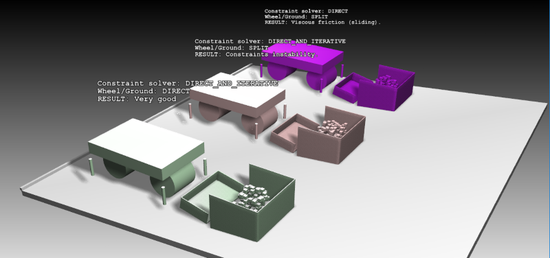
../_images/tutorial_iterative_and_direct.png

Fig. 9.4 Scene with three different solver configurations.¶

In the scene above there are three different set of vehicle/rocks. Each vehicle will drive forward, scoop up the “rocks” and back up and finally lift up the whole vehicle using the lifters in each corner.

Common for all of the three scenes are:

ITERATIVE contact solver is used between rocks (for scalability)
SPLIT contact solver is used between rocks and ground
SPLIT contact solver is used between rocks and the shovel

Differences between the scenes are:

Scene 1: (purple)

DIRECT solver is used for all ordinary constraints (Hinge, Prismatic etc.)
SPLIT contact solver is used between the lifter/wheels and the ground

Result: This scene demonstrates how the SPLIT solver will result in viscous friction due to the fact that the ITERATIVE solve for the friction is not accurate enough to resolve the frictional contact constraints.

Scene 2: (brown)

DIRECT_AND_ITERATIVE solver is used for all ordinary constraints.
SPLIT contact solver is used between the lifter/wheels and the ground.

Result: This scene demonstrate how the SPLIT solver in combination with DIRECT_AND_ITERATIVE constraint solver will result in unstable simulation. The error in the ITERATIVE part of contact solver will propagate to the ordinary constraints.

Scene 3: (green):

DIRECT_AND_ITERATIVE solver is used for all ordinary constraints.
DIRECT contact solver is used between the lifter/wheels and the ground.

Result: Here we get a stable simulation where all solvers are used in the best possible way. The ITERATIVE contact solver between rocks give good performance. The SPLIT solver between rocks and shovel and rocks and ground give good stability and acceptable performance. The DIRECT_AND_ITERATIVE solver for ordinary constraint will allow forces from the ITERATIVE system to propagate correctly to the DIRECT solver. The DIRECT solver between wheel/lifter and ground allow for stable and dry friction.

It would also be possible to use the ITERATIVE contact solver between rocks and the ground to improve performance. However, one possible artifact would be that the shovel could push the rocks into the ground/boxes due to large normal forces to which the ITERATIVE solver cannot handle correctly.