14. AGX Granular

14.1. Introduction

agx::Physics::GranularBodySystem is a extension of the agx::ParticleSystem class that contains spherical particles, called granular bodies, with 6 degrees of freedom (6-DOF) with Hertzian contact elasticity laws, Coulomb friction and rolling resistance. AGX Granular is based on a non-smooth dynamics formulation of the discrete element method (DEM) called non-smooth discrete element method (NDEM) 2. The granular system is solved together with the rest of AGX Dynamics which allows for a strong-coupling between articulated rigid body systems and granular bodies.

Note

In this chapter, the term particle and granular body ( or just body ) will be used interchangeably. They will all refer to the 6-DOF particle instance mentioned in the introduction above. A GranularBodyPtr is an extension of a ParticlePtr with additional buffers for inertia, rotation and angular velocity.

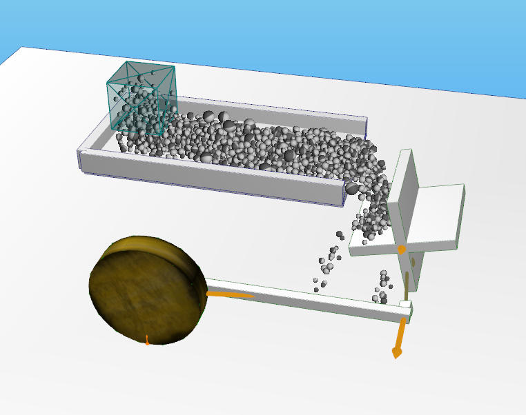
Figure 1: Example showcasing a granular body flow interacting with and driving a mechanical system of constrained rigid bodies.

A contact situation is illustrated in Fig 1. Contact forces and velocities can be decomposed in the direction of the contact normal \(\pmb{\vec{n}}\) and tangents \(\pmb{\vec{t}}\). The gap function \(g(\pmb{x})\) measures the magnitude of the overlap between the contacting bodies.

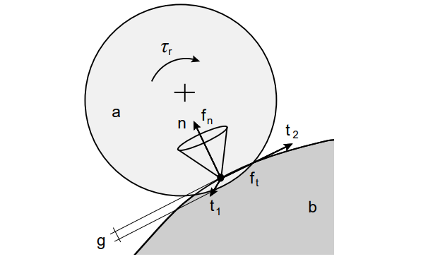
Figure 2: Illustration of a contact between two bodies \(a\) and \(b\) giving rise to a normal force \(f_n\), tangential force \(f_t\) and rolling resistance \(\tau_r\). The contact overlap is denoted by \(g\), the unit normal \(n\) and tangents \(t_1\) and \(t_2\).

agx::Physics::GranularBodySystem is used to simulate the movement of dynamic soil in agxTerrain.

14.1.1. Feature Overview

The GranularBodySystem contains memory-aligned attribute storages (position, velocity, inertia, etc… ) for increased efficiency and performance. Granular bodies have two-way interactions with all the other physical systems in AGX Dynamics, such as articulated multibody systems. GranularBody particles can be created from the system object or by using particle emitter. Particle distribution tables containing particle models with different radii and material properties can be used in the creation of particles. The large contact system that often results from granular body interaction can be solved using a parallel solver (PPGS) for increased performance where a warm starting option exist for increased solution fidelity. Particle states can also be written and read from files via the GranularReaderWriter class. The granular API is accessible via Python.

14.2. Basic Usage

14.2.1. Setup and Creation

The following code snippet demonstrates how to create a agx::Physics::GranularBodySystem system in C++:

// Create and configure a granular body system
agx::Physics::GranularBodySystemRef granularBodySystem = new agx::Physics::GranularBodySystem();
simulation->add( granularBodySystem );

Default values for created bodies can be set in the GranularBodySystem object:

// Properties set on the granularBodySystem are the default values of
// all created particles. These can of course be changed on an individual
// particle basis after creation.

// Most of the methods have optional arguments for updating existing particles
bool updateExistingParticles = false;

// Configure default values for created particles.
// When the radius is updated on particles, the mass is automatically calculated from
// the volume change.
granularBodySystem->setParticleRadius( 0.1, updateExistingParticles );

// Set the default agx::Material that governs body density and contact material.
// When the material is updated on particles, the mass is automatically calculated from
// the density in material->getBulkMaterial()->getDensity()
granularBodySystem->setMaterial( particleMaterial, updateExistingParticles );

Individial bodies can be created via the GranularBodySystem object. The body initially has default values but they can be changed after creation:

// Creation returns a agx::Physics::GranularBodyPtr representing the created particle
agx::Physics::GranularBodyPtr body = granularBodySystem->createParticle();

// Set position of the particle
body->setPosition( Vec3(0, 0, 4.5) );

// Set radius of particle ( updates mass )
body->setRadius( 0.1 );

// Set lifetime of particle in seconds
body->setLife( 2.0 );

// Set agx::Material of particle ( updates mass )
body->setMaterial( particleMaterial->getEntity() );

We can also create batches of bodies using bounds specified by the user:

// Create a bunch of particles in a bound.
agx::Bound3 spawnBound = agx::Bound3( Vec3(0.0, 0.0, 0), agx::Vec3(4.0, 1.0, 4.0) );

// The radius of all the created particles
agx::Real particleRadius = 0.1;

// Spacing between the created particles in the bound.
// Note that a spacing of 2 x radius will give a tight packing as
// particles will be placed next to eachother
agx::Vec3 spacing = agx::Vec3( radius * 2, radius * 2, radius * 2 );

// Add a random jitter on the placement of the particles. The jitterFactor is defined as
// the fraction of the specified particle spacing which will be used as the bound for
// the random perturbation of the particle placement.
agx::Real jitterFactor = 0.1;

// Place particles in an evenly spaced lattice 3D square lattice ( with jiter )
granularBodySystem->spawnParticlesInBound( bound, radius, spacing, jitterFactor );

// Place particles in a Hexagonal-Close-Packing (HCP) lattice
granularBodySystem->spawnParticlesInBoundHCP( bound, radius, spacing, jitterFactor );

Unless specified in the function call, the particles spawned carry default properties set in the agx:::Physics::GranularBodySystem object.

Deleting a granular body can be done in multiple ways, mainly via utiliy functions on the GranularBodySystem object:

// This will tag the particle for removal at the end of the timestep
// ensuring that it will be destroyed in a safe way.
// This can be called saftely any time during the timestep and is the
// recommended way of removing particles.
granularBodySystem->removeParticle( particle )

// You can check if a particle has been tagged for removed by checking it's state variable
// Option 1: via the particle instance
particle.state().removed()
// Option 2: via the granular system ( recommended ). Also checks if the particle instance
//           has been destroyed ( See below )
granularBodySystem->isValid( particle )

// This function immmediately destroys the particle instance.
// NOT recommended to do this in the middle of a simulation step since it
// will change the internal structure that can invalidate the simulation.
// ONLY do this after the simulation step in post() or last()
particle->destroy();

14.2.2. Motion Control

GranularBodies have a MotionControl state similar to RigidBodies. This can be set on bodies via a utility function on the GranularBodySystem object.

// Granular bodies support two MotionControls:
// 1. DYNAMICS - "Affected by forces, position/velocity is integrated by the *DynamicsSystem*."
// 2. KINEMATICS - "Not affected by forces, considered to have infinite mass. Velocities can be set by user."
// Make particle kinematic.
granularBodySystem->setMotionControl( particle, agx::Physics::GranularBodySystem::MotionControl::KINEMATICS )

// Particle will now effectivley have infinite mass. We now assign velocities to it.
particle->setVelocity( agx::Vec3( 1, 0, 0 ) ) // Set fixed translational speed in x-direction
particle->setAngularVelocity( agx::Vec3( 0, 0, agx::PI_2 ) ) // Rotational speed of 90 deg / s around z-axis

// Returns the motion control of the particle.
agx::Physics::GranularBodySystem::MotionControl particleMotionControl = granularBodySystem->getMotionControl( particle )

Note

In granular contacts where both granular bodies have the KINEMATICS motion control, the contact forces will not be calculated. This can be used to “freeze” areas of the simulation where particles are in rest in order to increase performance.

14.2.3. Access Granular Data

Regardless of how the granular bodies were created, individual particles can be accessed and manipulated using agx::Physics::GranularBodyPtrs; the same convention as with agx::ParticleSystem. A agx::Physics::GranularBodyPtr is an accessor object that gives access to the individual attributes of a granular body, stored as elements in the buffers that make up the EntityStorage that the particle in question is part of. The GranularBodyPtr exposes one method of access for each attribute of the GranularBody entities.

Table 14.1 Accessing Granular data

Position	getPosition/setPosition	Gets/Sets the position (agx::Vec3) of the body.
Rotation	getRotation/setRotation	Gets/Sets the rotation (agx::Quat) of the body.
Velocity	getVelocity/setVelocity	Gets/Sets the velocity (agx::Vec3) of the body.
Angular Velocity	getAngularVelocity/setAngularVelocity	Gets/Sets the angular velocity (agx::Vec3) of the body.
Force	getForce/setForce	Gets/Sets the force (agx::Vec3) acting on the body. Useful for using explicit force models on the bodies.
Mass	getMass/setMass	Gets/Sets the mass of the body. See note about automatic calculation below!
Inertia	getInertia/setInertia	Gets/Sets the inertia of the body. See note about automatic calculation below!
Life	getLife/setLife	Gets/Sets the lifetime of the particle in seconds.
Color	getColor/setColor	Gets/Sets the agxRender::Color (agx::Vec4f) of particle which is used in rendering.
Material	getMaterial/setMaterial	Gets/Sets the agx::Material of the particles which is used for determining contact material and in calculation of mass and density.

Note

Note that inertia and mass is automatically calculated when a agx::Material is assigned via the setMaterial function to the particle. If you want to manually edit these, be sure to do it after the agx::Material assignment.

agx::Real averageMass = 0.0;
agx::Real averageRadius = 0.0;
agx::MaterialRef newMaterial = new agx::Material( "newParticleMaterial" );
newMaterial->getBulkMaterial()->setDensiy( 1700 ); // kg/m3
granularBodies = granularBodySystem->getParticles();
for ( agx::Physics::GranularBodyPtr gPtr : granularBodies )
{
  gPtr->setVelocity( agx::Vec3( 0, 0, 0 ) );
  gPtr->setMaterial( newMaterial ); // This function updates the body mass from BulkMaterial density
  gPtr->setRadius( 0.05 ); // This function also updates the body mass
  averageMass += gPtr->getMass(); // extract the calculated mass
  averageRadius += gPtr->getRadius();
}

averageMass /= granularBodySystem->getNumParticles();
averageRadius /= granularBodySystem->getNumParticles();

14.3. Material Configuration and Parametrization

Physical properties and dynamic bulk behavior of the granular bodies are governed by the material settings and the contact material in the granular contacts. This section will cover the most important aspects of material parametrization to affect granular bulk behavior.

Particle density/mass is primary derived from the set agx::Material of the particle but can also be overridden manually:

// Set material density
agx::MaterialRef particleMaterial = new agx::Material( "particleMaterial" );
particleMaterial->getBulkMaterial()->setDensiy( 1700 ); // kg/m3

// Set the material as the default of granular bodies created from this system
// ( unless specified otherwise, e.g from a distribution table in an emitter )
granularBodysystem->setMaterial( particleMaterial );

// Manually create a particle and apply material to it
granularBodyPtr = granularBodysystem->createParticle();
granularBodyPtr->setMaterial( particleMaterial );

// Can also override this and apply a fixed mass. Not really recommended since
// material and radius assginment overries manually set mass values.
granularBodyPtr->setMass( 10 ); // kg

// Radius of the particle determines volume and thus resulting mass
granularBodyPtr->setRadius( 0.05 ); // m

In AGX Dynamics the constitutive equations in granular contacts follows Hertz contact law with Coulomb friction and rolling resistance 2. Contact material properties determines coefficients used in the contact laws where there are some unique parameters that are only active in granular contacts. The example below shows how to setup a contact material between granular bodies:

// Create new material that will be set to particle
agx::MaterialRef particleMaterial = new agx::Material( "particleMaterial" );
simulation->add( particleMaterial );
auto particleParticleCM = simulation->getMaterialManager()->getOrCreateContactMaterial( particleMaterial, particleMaterial );

// Apply the particle material to the granular body system so that it becomes the
// default material for new granular bodies
granularBodySystem->setMaterial( particleMaterial );

// Set the Young's Modulus of the contact material. In granular contacts, this corresponds
// direcly to Young's Modulus in Hertz contact law.
particleParticleCM->setYoungsModulus( 1e8 );

// The coulomb friction coefficient in the granular contacts
particleParticleCM->setFrictionCoefficient( 0.3 );

// The rolling resistance coefficients in the tangential direction of a contact
particleParticleCM->setRollingResistanceCoefficient( 0.3 );

// The twisting resistance coefficient in the normal direction of a contact
particleParticleCM->setTwistingResistanceCoefficient(0.001);

// The adhesive effects of the granular contacts. Determined by a max force in the adhesive
// contact as well as the depth overlap where the adhesive force is active
// Arguments are: max adhesive force ( N ), adhesive overlap ( m )
particleParticleCM->setAdhesion( 10, 0.05 );

// Set the restitution of the granular contact
particleParticleCM->setRestitution( 0.0 );

// Set the numerical damping of the contact
// In high timestep, it is usually some coefficient multiplied by the time step
particleParticleCM->setDamping( timeStep * 2 );

Note

The rolling and twisting resistance coefficients of the agx::ContactMaterial is unique to the granular <-> granular and granular <-> geometry contacts. They are not used in regular geometry and rigid body contacts.

14.4. Collision Groups

Collision groups can be set to the granular body system in order to configure collision settings in between particles and other geometries. These collision groups will be applied to all particles upon creation with optional argument for applying all existing instances as well.

// Optional argument for updating existing particles with the group
bool updateExistingParticles = false;

// Add collision group to system
granularBodySystem->addCollisionGroup( "group1", updateExistingParticles );

// Remove collision group from system
granularBodySystem->removeCollisionGroup( "group1", updateExistingParticles );

// Check if system has collision group ( expecting false )
granularBodySystem->hasCollisionGroup( "group1" );

Groups can be set on individual particles using the agx::Physics::GranularBodySystem interface:

// Add collision group to a single particle
agx::Physics::GranularBodyPtr ptr = granularBodySystem->createParticle()
granularBodySystem->addCollisionGroupParticle( "group1", ptr );

// Remove collision group from GranularBody
granularBodySystem->removeCollisionGroupParticle( "group1", ptr );

// Check if particle has collision group ( expecting false )
granularBodySystem->hasCollisionGroupParticle( "group1", ptr );

You can also disable collision between particles and specific geometries:

// geometry argument is a agxCollide::Geometry
granularBodySystem->setEnableCollisions( geometry, false );

14.5. Particle Distribution Tables

Particle distribution tables are used to represent distributions of particle types with different properties such as radii and material. The agx::EmitterDistributionTable is a base class in the agx::Emitter class and can be used for particle distributions in Particle emitters or for rigid body distributions in RigidBody emitters.

Distribution tables contains a set of different particle distribution models. A distribution model consists of a radius, an agx::Material and a weight. The weight is the probability to create a particle of the corresponding model when the table is queried of a random model.

The user specifies a agx::Emitter::Quantity when a distributions table is created. This quantity is the basis of the probability of how particle models should be selected with respect to their weight. If a model has a higher weight relative to the other models in a table it will contribute more to the total amount of created quantity ( number of particles, mass or volume ) from that table.

Table 14.2 Different quantity settings of the distribution table

QUANTITY_COUNT	Counting number of individual particles as the quantity.
QUANTITY_VOLUME	Counting the total volume of emitted particles as the quantity.
QUANTITY_MASS	Counting the total mass of the emitted particles as the quantity.

Example:

The quantity is set to QUANTITY_MASS and the table contains two models, one that has weight 1 and the other weight 2. Then the probability of particle creation is set so that the second model will contribute two times more mass than the first model to the total mass that is created from the table. If QUANTITY_COUNT is set, then the second model will yield twice as many discrete elements as the first one of the total amount of particles created from the table.

// Create a new distribution table with specified quantity
agx::Emitter::DistributionTableRef table = new agx::Emitter::DistributionTable( agx::Emitter::QUANTITY_MASS )

// Arguments to a particle model is: radius, agx::Material, weight
table->addModel( new agx::ParticleEmitter::DistributionModel( 0.05, pelletmat, 0.3 ) )
table->addModel( new agx::ParticleEmitter::DistributionModel( 0.09, pelletmat, 0.6 ) )
table->addModel( new agx::ParticleEmitter::DistributionModel( 0.15, pelletmat, 0.1 ) )

Random models can be queried from the table using the following call:

// Query the table for a random model
DistributionModel* model = distributionTable->getRandomModel();

// Since this will return an abstract model ( particle and rigid body models are subclasses ),
// we need to cast it to a particle model
agx::ParticleEmitter::DistributionModel* particleModel = model->as< agx::ParticleEmitter::DistributionModel >();

Distribution tables are used both in particle emitters and when creating batches of particles.

14.6. Particle Emitter

The agx::ParticleEmitter is used to continuously create a stream of particles in a predefined volume defined by a agxCollide::Geometry. The created particles carry the default properties of the coupled granularBodySystem, with the exception of color and life which can be set individually per emitter.

Note

In order to create emitters that emits bodies/particles with different materials, see Distribution tables

// When a particle emitter is created, it needs to be coupled to a existing ParticleSystem/granularBodySystem.
agx::ParticleEmitterRef emitter = agx::ParticleEmitter( granularBodySystem );

// Set the geometry that will server as a spawning volume for the particles
emitter->setGeometry( agxCollide::Geometry( agxCollide::Cylinder( 1.6, 10 ) ) );

// Add the emitter to the simulation to connect it's update task to the simulation
simulation->add( emitter );

Note

The emitter agxCollide::Geometry acts just like any other geometry. You can add it to a body in order to create a dynamically moving emitter.

A Quantity needs to be assigned to an emitter to determine the nature of the creation, similar in creation of particle distribution tables. This determines if the given creation rate is based on discrete number of particles, mass or volume.

emitter->setQuantity( agx::Emitter::Quantity::COUNT );

The emitter contains a parameter to control the rate of the particle creation which is dependent on current set quantity of the emitter.

emitter->setRate( 15 );

The maximum amount of quantity ( num particles, mass or volume ) that can be emitted can be adjusted:

/**
What the set amount means depends on the current Quantity setting of the emitter.
QUANTITY_COUNT  - max number of objects
QUANTITY_VOLUME - max total volume of objects
QUANTITY_MASS   - max total mass of objects
*/
emitter->setMaximumEmittedQuantity( 15 );

You can get information about emitted quantity and the number of particles emitted:

/**
* Returns the quantity amount of that this emitter has emitted.
*/
emitter->getEmittedQuantity() const;

/**
\return the number of bodies that this emitter has emitted
*/
emitter->getNumEmitted() const;

Distribution tables can be used in emitters by a simple assignment:

emitter->setDistributionTable( particle_table );

It will then query the table for a particle model when creating new elements instead of using the default settings in the coupled GranularBodySystem.

Collision Groups of emitted particles can also be adjusted on an emitter basis. These groups are added on top of the groups that has been added via the granular body system object:

emitter->addCollisionGroup( "emitter_group" );
emitter->removeCollisionGroup( "emitter_group" );
bool hasGroup = emitter ->hasCollisionGroup( "emitter_group" );

The life parameter of particles can also be set on an emitter basis.

emitter->setLife( 10 );

Initial velocity of created particles can also be set via the emitter:

emitter->setVelocity( agx::Vec3( 1, 1, 1 ) );

14.7. Granular Bodies in Python

The functionality around GranularBodySystem and particle emitters can be used via the Python API.

Note

Due to the SWIG mapping the subclass namespace structure in C++ is compressed in the resulting Python API. This primary affects the distribution table, particle model and the GranularBodySystem classes.

Table 14.3 Table showing the SWIG mapping of the Granular C++ API to Python API

C++ API	Python API
agx::Physics::GranularBodySystem	agx.GranularBodySystem
agx::Emitter::DistributionTable	agx.EmitterDistributionTable
agx::ParticleEmitter::DistributionModel	agx.ParticleEmitterDistributionModel

The following code snippet demonstrates how to create a simple granular body system in Python and some example applications for creating bodies.

# Create and configure a particle system.
granular_body_system = agx.GranularBodySystem()
sim.add( granular_body_system )
granular_body_system.setMaterial( granularMaterial )

# Create a single particle.
gBodyPtr = granular_body_system.createParticle()
gBodyPtr.setPosition( agx.Vec3( 0, 0, 4.5 ) )

# Create a bunch of particles in a bound.
particle_radius = 0.1
spawn_bound = agx.Bound3( agx.Vec3(0, 0, 0), agx.Vec3(4,1,4) )
granular_body_system.spawnParticlesInBound( spawn_bound, particle_radius, agx.Vec3( particle_radius * 2 ) )

Sample code for setting up a DistributionTable:

# Create a new distribution table with specified quantity
table = agx.EmitterDistributionTable( agx.Emitter.QUANTITY_MASS )

# Arguments to a particle model is: radius, agx::Material, weight
table.addModel(agx.ParticleEmitterDistributionModel( 0.05, pelletmat, 0.3 ) )
table.addModel(agx.ParticleEmitterDistributionModel( 0.09, pelletmat, 0.6 ) )
table.addModel(agx.ParticleEmitterDistributionModel( 0.15, pelletmat, 0.1 ) )

Emitters can also be created in Python:

# init emitter with mass quantity setting
emitter = agx.ParticleEmitter( granularBodySystem, agx.Emitter.QUANTITY_MASS )

# Set the previously declared distribution table to the emitter.
emitter.setDistributionTable( table )
emitter.setRate( 15 ) # 15 kg/s
emitter.setMaximumEmittedQuantity( 100 ) # 100kg

# Create spawn geometry for the emitter. The particles will be created inside the bound of the coupled geometry.
emitterSize = agx.Vec3( 0.5, 0.5, 0.5 )
emitterGeom = agxCollide.Geometry( agxCollide.Box( emitterSize ) )
emitterGeom.setPosition( g_emitterSpecification[ "position" ] )

# Disable collisions in emitter to remove contacts with the particles created in the volume.
emitterGeom.setEnableCollisions( False )
sim.add( emitterGeom )
emitter.setGeometry( emitterGeom )

# Set an initial velocity downward
emitter.setVelocity( agx.Vec3( 0 , 0, -1.0 ) )
sim.add( emitter )

14.8. Extract contact data in Python

Contact data involving granular bodies can be extracted via agxCollide::Space. The following snippet showcases how to extract and read:

Warning

Contact normals and tangents are in agx.Vec3f format. They need to be converted to agx.Vec3 in order to be used in multiplication with other data in the agx.Vec3 format that is returned from functions like getPosition() and getVelocity().

# Extract particle <-> particle contacts
particle_particle_contacts = sim.getSpace().getParticleParticleContacts()
for c in particle_particle_contacts:
    # Get particle ids from the contact
    id_particle1 = c.getParticleId1()
    id_particle2 = c.getParticleId2()

    # Get ParticlePtr/GranularBodyPtr from ids by using the GranularBodySystem
    p1 = granularBodySystem.getParticle(id_particle1)
    p2 = granularBodySystem.getParticle(id_particle2)

    # Get normals and tangents. These are all in agx.Vec3f format
    # they need to be converted to agx.Vec3 in order to be multiplied with
    # agx.Vec3 from methods like 'getVelocity' or 'getPosition'
    normal = c.getNormal()
    tu = c.getTangentU()
    tv = c.getTangentV()

    # Extract contact force. Note that this will be zero if read in the
    # 'pre-step' phase of the simulation. Forces are available in the
    # 'post-step' phase of the simulation which is executed after the solver.
    f = c.getLocalForce()

    # Get contact point and depth
    point = c.getPoint()
    depth = c.getDepth()

# Extract particle <-> geometry contacts
particle_geometry_contacts = sim.getSpace().getParticleGeometryContacts()
for c in particle_geometry_contacts:
    # Get particle id in the contact
    id_particle = c.getParticleId()

    # Get ParticlePtr/GranularBodyPtr from id by using the GranularBodySystem
    p = granularBodySystem.getParticle(id_particle)

    # Get the geometry from the contact and then it's rigid body, if it exists
    id_geometry = c.getGeometryId()
    geom = sim.getSpace().getGeometr(id_geometry)
    # Will return None if geometry has no rigid body
    rigidBody = geom.getRigidBody()

    # Get normals and tangents. These are all in agx.Vec3f format
    # they need to be converted to agx.Vec3 in order to be multiplied with
    # agx.Vec3 from methods like 'getVelocity' or 'getPosition'
    normal = c.getNormal()
    tangentU = c.getTangentU()
    tangentV = c.getTangentV()

    # Extract contact force. Note that this will be zero if read in the
    # 'pre-step' phase of the simulation. Forces are available in the
    # 'post-step' phase of the simulation which is executed after the solver.
    f = c.getLocalForce()

    # Get contact point and depth
    point = c.getPoint()
    depth = c.getDepth()

Existsing Python tutorials goes further in showcasing GranularBodySystem functionality.

14.9. Solver Settings

Solver settings affect the performance and fidelity of GranularBodySystem. Every granular contact is solved using an iterative solver configuration; The typical large contact network that results from big granular systems quickly become unfeasible for a direct solver.

Note

GranularBodySystem particle <-> particle and particle <-> geometry contacts are ALWAYS solved using an iterative solver for all the 6 contact equations ( 1 x normal, 2 x friction, 2 x tangential rolling resistance and 1 x twisting resistance ). Contact material Friction model settings have no effect on this.

A basic setup of the solver can look like this:

// Set maximum amount of threads for usage in the parallel solver
// We prefferable want to use a number of threads equal to number of physical
// cores present in the machine. So account for potential HT/SMT.
agx::setNumThreads( 0 );
int n = agx::getNumThreads() / 2; // Account for hyper-threading
agx::setNumThreads( n );

// Apply simulation solver parameters.
// Use the parallel PGS solver for best performance using multiple threads.
sim->getDynamicsSystem()->getSolver()->setUseParallelPgs( true )

// Enable 32bit float solver for granular bodies to increase performance.
sim.getDynamicsSystem()->getSolver()->setUse32bitGranularBodySolver( true );

// Enable granular warm starting for all solver configurations to enable better solutions.
sim->getDynamicsSystem()->getSolver()->setUseGranularWarmStarting( true );

// Set number of iterations that should be used in the Parallel Gauss-Seidel Solver.
// The higher number the better solution, but will also impact performance.
sim->getDynamicsSystem()->getSolver()->setNumPPGSRestingIterations( 50 );

// Set the number of resting iterations in the regular serial iterative solver.
// Higher iterations result in better solutions with increaded computational cost.
sim->getDynamicsSystem()->getSolver()->setNumRestingIterations( 50 );

14.9.1. Parallel Projected Gauss Seidel (PPGS)

The contact system can be solved by a Parallel-Projected Gauss-Seidel Solver (PPGS). The solver first partitions the system into different subdomains and interaction zones that are solved in parallel via multithreading. The iteration count used in the solver can be adjusted according to fidelity needs.

Solver settings can be adjusted to increase or decrease simulation fidelity with respect to computational performance.

// Use the parallel PGS solver for best performance using multiple threads
sim->getDynamicsSystem()->getSolver()->setUseParallelPgs( true )

// Set number of iterations that should be used in the Parallel Gauss-Seidel Solver.
// The higher number the better solution, but will also impact performance.
sim->getDynamicsSystem()->getSolver()->setNumPPGSRestingIterations( 50 )

Note

PPGS can be used for rigid body contacts as well. When enabled every rigid body contact with a contact material that has the agx::IterativeProjectedConeFriction( agx::FrictionModel::ITERATIVE) as set Friction Model will be included in the PPGS solver.

14.9.2. Warm Starting Granular Contacts

The PPGS solver can be warm-started by using the constraint multiplier lambda ( \(\lambda\) ) from the solution of the contact constraint equations in the previous time-step. In general, this will enable contacts that persists over time to converge faster and result in a more precise solution of PPGS solver with fewer number of iterations. This option is recommended when simulating slowly evolving systems with contact networks. For rapidly evolving systems, there is little benefit from using warm-starting or even risk that it worsen the convergence.

// Enable granular warm starting for all solver configurations to enable better solutions
sim->getDynamicsSystem()->getSolver()->setUseGranularWarmStarting( true )

14.9.3. 32bit Granular Solver

The iterative solvers that are used when solving the granular contact networks always has some error. The order of magnitude of the error is in all cases higher than the precision of 64it floats. Due to this fact there exists an option of only using 32bit floats in the granular solver to increase compute performance by up to 30-40%.

// Enable granular warm starting for all solver configurations to enable better solutions
sim->getDynamicsSystem()->getSolver()->setUseGranularWarmStarting( true )

14.10. GranularReaderWriter

GranularBodySystem and particle data can be serialized and stored separately apart from the regular serialization functionality of AGX Dynamics using the agx::GranularReaderWriter class. This can be used to store granular data in .agx, .aagx and .csv.

// Extension of filename determines the file format that is stored ( .agx, .aagx or .csv )
std::string filename = "particles.agx";

// Vector of GranularBodyPtr:s, can be individually picked. Can also store every body by
// extracting them via the getParticles() function
agx::Physics::GranularBodyPtrVector bodies = granularBodySystem.getParticles();

// Optional argument transform is applied to the position and velocity
// of the bodies before storing to file.
// Create simple translation matrix in this case
agx::AffineMatrix4x4 transform = agx::AffineMatrix4x4::translate( 0, 1, 2 );

// Write all the existing bodies to an .agx file
agx::GranularReaderWriter::writeFile( filename,
                                      bodies,
                                      granularBodySystem,
                                      transform );

We can then load stored bodies from an .agx file:

// Specify the .agx file to load bodies from
std::string filename = "particles.agx";

// Vector of GranularBodyPtr:s where the loaded bodies will be inserted
agx::Physics::GranularBodyPtrVector granularBodies;

// Optional argument transform is applied to the position and velocity
// of the bodies before loading into the simulation.
// In this case, we want to invert the previous translation matrix to bring the bodies back to the origin frame.
agx::AffineMatrix4x4 transform = agx::AffineMatrix4x4::translate( 0, 1, 2 ).inverse();

// Load the bodies from the specified filename
bool success =  loadFileAGX( filename,
                             granularBodies, // loaded bodies will be inserted into this vector
                             granularBodySystem, // loaded bodies will be inserted into this granular body system
                             transform );

References

1

3. Lacoursière, Regularized, stabilized, variational methods for multibodies, in: D.F. Peter Bunus, C. Führer (Eds.), The 48th Scandinavian Conference on Simulation and Modeling (SIMS 2007), Linköping University Electronic Press 2007, pp. 40–48

2(1,2)

Wang, D. (2015). Accelerated granular matter simulation (PhD dissertation). Umeå. pdf.

14.11. RigidBody emitter

An agx::RigidBodyEmitter creates new rigid bodies at a certain rate within a specified volume and adds them to the simulation. This is useful when you do not want to create all the rigid bodies at the start of the simulation and/or when the rigid bodies in your simulation should follow some kind of size/shape distribution.

The following code snippet demonstrates how to create a rigid body emitter in c++:

agx::RigidBodyEmitterRef emitter = new agx::RigidBodyEmitter();
emitter->setRate(30.0);
emitter->setMaximumEmittedQuantity(200);
emitter->setQuantity(agx::Emitter::QUANTITY_COUNT);

The rate and the maximumEmittedQuantity decides how fast the emitter creates new bodies and what the maximum quantity is. There are three different ways of counting the quantity of the emitter.

Table 14.4 Different quantity settings of the emitter and distribution table

QUANTITY_COUNT	Counting number of individual rocks as the quantity.
QUANTITY_VOLUME	Counting the total volume of emitted rocks as the quantity.
QUANTITY_MASS	Counting the total mass of the emitted rocks as the quantity.

When the emitter creates a new rigid body it randomly chooses a distributionModel from the distributionTable. A distributionModel consists of a rigidBody template and a weight. The weight is the probability to create a clone of the corresponding rigid body template and adding it to the simulation. By adding several different distributionModels to the distributionTable of the rigid body emitter, the same emitter can emit rigid bodies with different geometries, sizes and materials. A short code example on how to create a distributionTable with one distributionModel:

// Create distribution table
agx::Emitter::DistributionTableRef distributionTable = new agx::Emitter::DistributionTable(agx::Emitter::Quantity::QUANTITY_MASS);

// Create template
agx::RigidBodyRef bodyTemplate1 = new agx::RigidBody();
agxCollide::GeometryRef geometryTemplate1 = new agxCollide::Geometry(new agxCollide::Cylinder(0.4, 0.1));
geometryTemplate1->setMaterial(material);
bodyTemplate1->add(geometryTemplate1);

distributionTable->addModel(new agx::RigidBodyEmitter::DistributionModel(bodyTemplate1, 0.3));
emitter->setDistributionTable(distributionTable);

Finally the rigidBodyEmitter needs a volume in which rigid bodies will spawn. It is defined as an agxCollide::Geometry:

agxCollide::GeometryRef emitGeometry = new agxCollide::Geometry(new agxCollide::Sphere(3.0));
emitGeometry->setSensor(true);
emitter->setGeometry(emitGeometry);