33. Robotics
AGX dynamics offers flexibility in simulating robotics for various tasks and seamless integration with other software.
Robots based on CAD drawings or URDF can be imported and configured in Python or C++.
Once the model is in place, AGX supports motion planning, testing, developing, and training controllers through reinforcement learning.
The controller can live directly in AGX or elsewhere and communicate with the simulation using middleware such as ROS2.
33.1. Serial chains
Although AGX dynamics supports modelling all types of robot mechanisms, the most convenient way to do conventional robotics is to use a agxModel::SerialKinematicChain.
It offers functionality for planning and control, including forward, inverse, and differential kinematics, as well as forward and inverse dynamics.
A kinematic chain is a description of a mechanical system. The chain links are rigid bodies that are constrained to each other. Depending on its topology, a chain is classified as either serial, tree, or graph structure. Serial chains and trees are open without loops, whereas the graph can be closed. A serial kinematic chain describes many mechanisms, such as industrial robots, excavator arms, and cranes.
The class agxModel::SerialKinematicChain in AGX represents an open serial chain.
There are two ways to initialize this class.
The first is to provide a simulation along with the base and end bodies, in which case the implementation searches through the simulation breadth first among the bodies and constraints.
The other way to create a chain is to provide a list of bodies and a list of constraints.
In this case, the items’ order in both lists is crucial to create a valid chain as it requires that constraint[i] connects body[i] and body[i+1].
33.1.1. Forward kinematics
Forward kinematics is concerned with finding the position and orientation of the end-effector, given the robot’s joint configuration. In the case of serial chains, joint configurations respecting limits result in valid end-effector poses in the task space.
AGX dynamics supports computing forward kinematics relative to the base from a agxModel::SerialKinematicChain.
The method computeForwardKinematics computes an AffineMatrix4x4 pose of the end-effector given a joint configuration, including the option to consider joint limits.
Similarly, computeForwardKinematicsAll computes the pose of all links in a chain.
Examples of forward computations can be seen in data/python/tutorials/RobotControl/tutorial_set_robot_pose.agxPy.
33.1.2. Manipulator Jacobian
The manipulator Jacobian \(J(q)\) is a component of differential kinematics and essential for controlling and planning the motion of robotic manipulators. It relates the joint velocities \(\dot{q}\) with the velocity of the end-effector \(v\) according to
The method computeManipulatorJacobian evaluates the manipulator Jacobian in fixed frame coordinates relative to the base.
It takes the joint positions \(q\) as input and outputs the Jacobian matrix stored by row in a vector with size \(6 \times N_j\).
33.1.3. Inverse kinematics
Inverse kinematics (IK) deals with finding joint configurations that correspond to the desired position and orientation of the end-effector in task space. Unlike forward kinematics, the inverse problem can have zero, multiple, or infinitely many solutions. If the desired pose is unreachable by the manipulator, IK has zero solutions. When a robot has more joints than the dimension of the task space, it is called redundant. While multiple solutions may exist for nonredundant manipulators, e.g. in the case of elbow up or elbow down, only redundant robots can have infinitely many solutions.
A general approach to solve the IK problem for open chains is to rely on iterative numerical algorithms. These take advantage of the inverse of the manipulator Jacobian to find a solution when one exists.
The agxModel:SerialKinematicChain can compute IK via the method computeInverseKinematics.
The input is a desired end-effector transform in task space relative to the base, current joint positions to help guide the algorithm toward a solution, and an optional solver tolerance.
We recommend checking the IK computations return status (enum) before using the output joint angles. Also, the best practice is to use the latest joint positions as an initial guess. This is to avoid cases where a slight change in end-effector transform causes an element in the output joint position to switch from \(\pi\) to \(-\pi\).
33.1.4. Inverse dynamics
Dynamics is the study of motions and the forces and torques that cause them. AGX typically follows this process: Advancing the simulation based on current forces and torques acting on bodies and particles, resulting in a new state with updated positions and velocities.
The problem of inverse dynamics (ID) is to find the forces/torques that result in a certain state. This is the opposite of forward dynamics, where the forces and torques are known, but the new state is not.
Unlike kinematics computations, inverse dynamics computations in the SerialKinematicChain require knowledge of the simulation.
Therefore, the chain must receive a simulation instance either through the constructor or by invoking setSimulation at a later stage.
With knowledge of the simulation, computeInverseDynamics performs the ID computations with an input corresponding to the desired joint accelerations, \(\ddot{q}_\mathrm{desired}\).
The rest of the state, current \(q\) and \(\dot{q}\) are available via the simulation.
The computed output is a vector with forces/torques \(\tau\).
One overload to computeInverseDynamics also accepts additional external forces acting on the chain’s links.
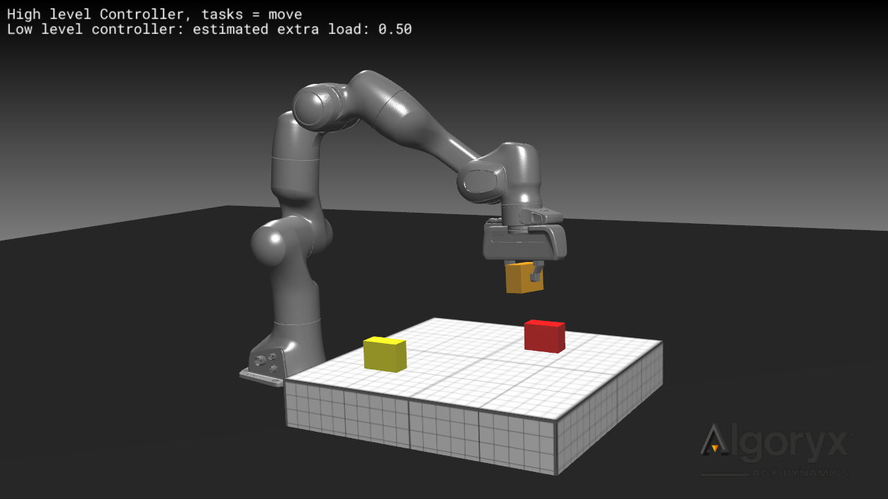
Examples with ID including external forces are available both in python data/python/tutorials/RobotControl/tutorial_pick_and_place.agxPy and C++ tutorials/agxOSG/tutorial_robot_pick_and_place.cpp.
Ensure thread safety when using computeInverseDynamics.
The method reads data from the chain’s components and transforms constraint attachment frames.
Therefore, calling this method from a separate thread while the solver runs in another may cause incorrect results or undefined behaviour.
Instead, recommended use is between calls to Simulation::stepForward or within a StepEventListener callback method, such as pre or preCollide.
33.2. Robot control
How to control a robot to achieve the desired behaviour depends on the working environment and the task tries to solve. AGX Dynamics aims to provide functionality that makes it easy to test, develop, and train controllers in dynamic simulation environments for various applications.
33.2.1. PID control
The most basic controller is the Proportional-Integral-Derivative (PID) controller. As a PID lacks a dynamic model of the robot, control relies entirely on feedback. The following mathematical expression describes it:
where \(u\) is the output signal, also known as the Manipulated Variable (MV), \(e\) is the error between the measured process variable and the set point, and \(K_p\), \(K_i\), and \(K_d\) are the tuning parameters, or proportional gain, integral gain, and derivative gain.
A PID controller can be used on its own or as part of a controller. For more details about the PID implementation in AGX and examples of PID control, see AGX Model: PID Controller.
33.2.2. Velocity control
Although most robots use actuators with force or torque inputs, these may be set to velocity mode for control. Velocity mode means that the velocities of the joints are controlled directly.
In AGX dynamics, joints are modelled as constraints with a single degree of freedom, i.e. either as a agx::Hinge or agx::Prismatic.
These constraints can activate a agx::Motor1D, which allows setting a desired joint velocity through the setSpeed method.
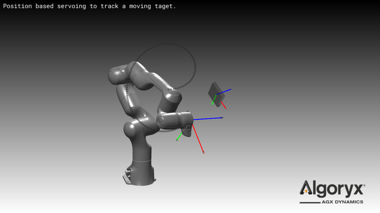
The tutorial data/python/tutorials/RobotControl/tutorial_differential_kinematics.agxPy demonstrates velocity control of the Franka Emika Panda when the task is to track a moving object.
In the tutorial, we implement a control method called Position-based servoing, which relies on the pseudoinverse of the manipulator Jacobian to compute joint velocities.
33.2.3. Torque control
In contrast to calculating torques using a PID controller, precise torque control requires a dynamics model of the robot.
When a dynamics model is at hand, inverse dynamics calculates the torques that achieve a desired motion.
For instance, the tutorial data/python/tutorials/RobotControl/tutorial_gravity_compensation.agxPy demonstrates how to counteract gravity and maintain zero acceleration.
However, as no model is perfect, most practical controllers rely on feedback.
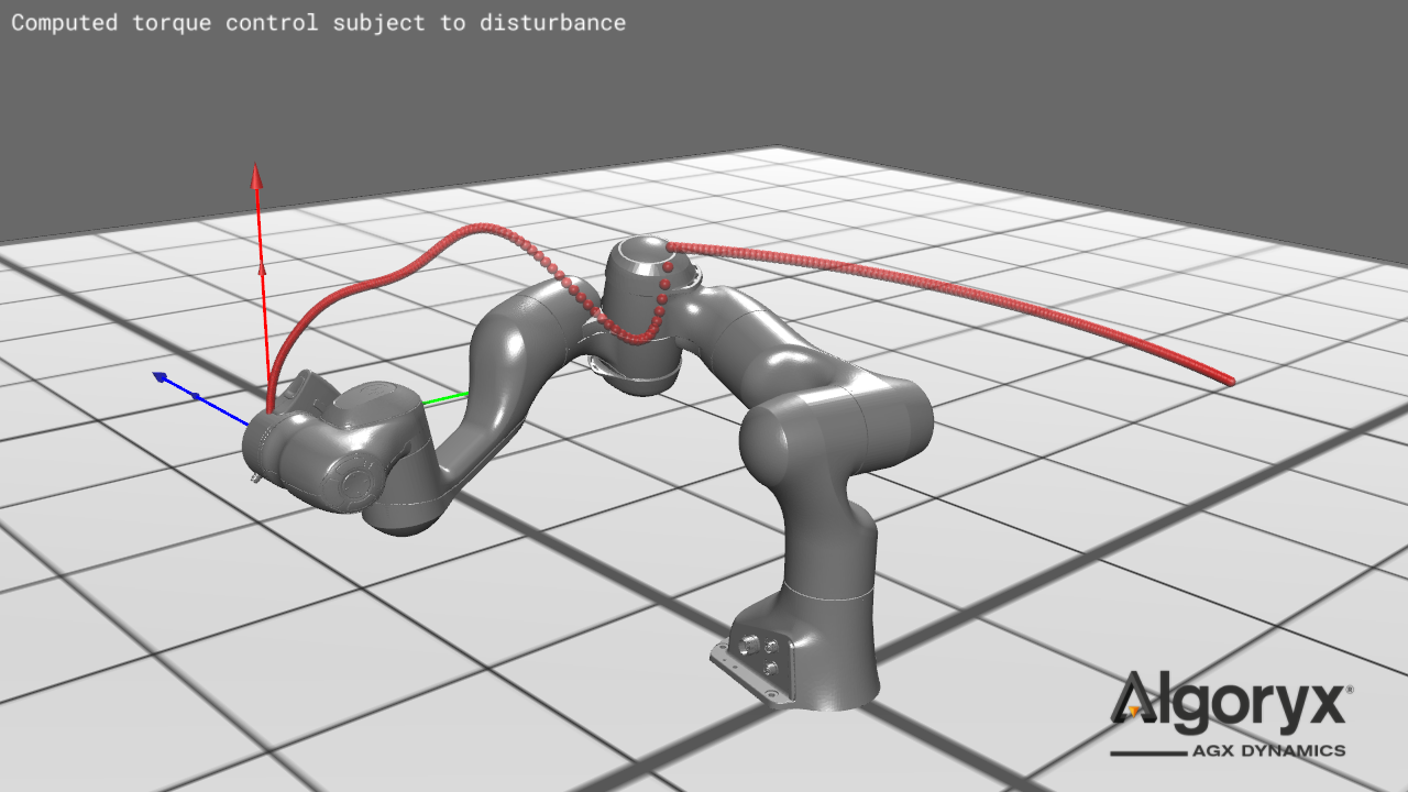
A motion control algorithm that combines feed-forward with feedback is computed torque control as demonstrated in data/python/tutorials/RobotControl/tutorial_computed_torque_control.agxPy.
Regardless of where the desired torques come from, a simple way to torque-control a robot in AGX dynamics is to use a agx::Motor1D on each joint.
An agx::Motor1D achieves the desired torque tau by setting the same value to the upper and lower limit through setForceRange(tau, tau).
For more accurate modelling of the actuator dynamics, refer to AGX DriveTrain.
However, agx::DriveTrain is currently not supported by computeInverseDynamics but is expected to be so in the near future.
33.3. ROS2
The Robot Operating System (ROS) is a middleware and framework that is often used to work with robotics. It is not an Operating System even if the name implies so. One fundamental part in ROS2 is message-passing between different nodes, for example a controller that could be sending and receiveing messages for a real or virtual robot.
ROS2 support in AGX Dynamics comes in two levels:
AGX Dynamics built in ROS2 support (see Built in ROS2 support for details).
Always available in AGX Dynamics on all supported operating systems except Ubuntu 18.04.
Publisher / Subscriber message passing support.
Supports all message types in
std_msgs,sensor_msgs,builtin_interfaces,rosgraph_msgs,geometry_msgsandagx_msgs.Mechanism for serialization / deserialization of custom types (see Using custom types for details).
QOS and domain ID support.
No user-defined ROS2 package compilation support.
Pre-built ROS2 installation (see Pre-built ROS2 installation for details).
Available for Windows only.
Can be used together with AGX Dynamics in Python environments.
User defined ROS2 packages can be compiled and used.
Several built in ROS2 features that come with a typical ROS2 installation.
33.3.1. Built in ROS2 support
With AGX Dynamics it is possible to do Publisher / Subscribe message passing. It does not require a separate ROS2 installation or build in order to work.
All messages types in the following packages are supported:
std_msgs, sensor_msgs, builtin_interfaces, rosgraph_msgs, geometry_msgs and agx_msgs.
AGX Dynamics offers an API through the agxROS2 namespace that wraps some of the ROS2 functionality, namely Publisher and Subscriber message passing.
Specifying QOS such as reliability, durability, history type and depth as well as domain ID is also supported.
It targets the version ROS2 Humble and specifically the DDS implementation Fast-DDS which is the default DDS implementation in ROS2 Humble.
ROS2 generally does not guarantee compatibility between ROS2 versions and DDS vendors, but it should work in practice, especially when matching the DDS vendor types.
For more details regarding specifying the DDS vendor in a ROS2 environment, see Troubleshooting.
The built in ROS2 support does not support compiling and using user defined message types, but there is a mechanism avaiable to enable sending and receiving custom data types, see Using custom types for details.
Below are two minimal examples of how to create a Publisher and Subscriber through the built in ROS2 support and passing a message between them. Note that the Publisher and Subscriber code normally are run on two separate applications and/or computers.
In C++:
#include <agxROS2/Publisher.h>
#include <agxROS2/Subscriber.h>
#include <iostream>

int main()
{
  // Create Publisher and Subscriber with specific Topic.
  agxROS2::stdMsgs::PublisherFloat32 pub("my_topic");
  agxROS2::stdMsgs::SubscriberFloat32 sub("my_topic");

  // Create a message and send it.
  agxROS2::stdMsgs::Float32 msgSend;
  msgSend.data = 3.141592f;
  pub.sendMessage(msgSend);

  // Try to receive the message.
  agxROS2::stdMsgs::Float32 msgReceive;
  if (sub.receiveMessage(msgReceive))
    std::cout << "Received message: " << msgReceive.data << ".\n";
  else
    std::cout << "Did not receive a message.\n";

  return 0;
}
In Python:
import agxROS2

def main():
    # Create Publisher and Subscriber with specific Topic.
    pub = agxROS2.PublisherStdMsgsFloat32("my_topic")
    sub = agxROS2.SubscriberStdMsgsFloat32("my_topic")

    # Create a message and send it.
    msgSend = agxROS2.StdMsgsFloat32()
    msgSend.data = 3.141592
    pub.sendMessage(msgSend)

    # Try to receive the message.
    msgReceive = agxROS2.StdMsgsFloat32()
    if sub.receiveMessage(msgReceive):
        print("Received message: {}".format(msgReceive.data))
    else:
        print("Did not receive a message.")

if __name__ == '__main__':
    main()
More advanced usage such as using a specific QOS or custom types can be seen in the tutorial tutorials/agxOSG/tutorial_ros2.cpp.
33.3.1.1. ros2_control interface
ros2_control is a commonly used framework to control robots using ROS2. You can find the documentation to ros2_control (here).
We provide an easy way to communicate with ros2_control controllers using class ROS2ControlInterface which inherits from agxSDK::StepEventListener. It assumes that
the joint commands and states is communicated on ROS2 topics using the sensor_msgs/msg/JointState message type. And that the robot loaded into ros2_control
uses the (topic_based_ros2_control) hardware interface configured to
use the same topics.
// Read your robot urdf file
agxSDK::AssemblyRef model = agxModel::UrdfReader::read(urdfFile, urdfPackage, initialPositions.get(), settings);

// Create the ROS2ControlInterface StepEventListener with set ROS2 topics for commands and states
auto ros2ControlInterface = agxROS2::ROS2ControlInterface("joint_commands", "joint_states");

// Add the 1DOF contraints from the robot you want to control and how you want to control it
ros2ControlInterface.addJoint(model->getConstraint1DOF("joint1"), agxROS2::ROS2ControlInterface::POSITION)
ros2ControlInterface.addJoint(model->getConstraint1DOF("joint2"), agxROS2::ROS2ControlInterface::POSITION)

// Add the listener to the simulation
simulation->add(ros2ControlInterface)
Or in python with
# Create an excavator
  excavator = Excavator()

  excavator.setRotation(terrain.getRotation())
  excavator.setPosition(0, 0, 0)
  simulation().add(excavator)

  joint_names = [
      'ArticulatedArm_Prismatic',
      'ArmPrismatic',
      'StickPrismatic',
      'TiltPrismatic',
      'BucketPrismatic',
      'BladePrismatic1',
      'BladePrismatic2',
      'CabinHinge',
      'LeftSprocketHinge',
      'RightSprocketHinge',
  ]

  excavator_ros2_interface = agxROS2.ROS2ControlInterface(
      "joint_commands",
      "joint_states",
  )
  for name in joint_names:
      excavator_ros2_interface.addJoint(excavator.getConstraint1DOF(name), agxROS2.ROS2ControlInterface.VELOCITY)
33.3.1.2. PointCloud2 usage with agxSensor
The sensorMsgs/PointCloud2 message type (avaiable using the built in support for ROS2 in AGX) defined in the sensorMsgs module for ROS2 provides a standardized type for point clouds but the output produced by the raytracing library used for our lidar solution (see Lidar) is not directly compatible with this message format. To simplify sending lidar output over ROS2 a utility function agxROS2::convertLidarOutput defined in agxROS2/ROS2Util.h is provided.
// Converts an output recieved from a lidar's output handler into a ROS2 message ready for publishing
agxROS2::sensorMsgs::PointCloud2 convertLidarOutput(agxSensor::RtOutput* lidarOutput, double timestamp, std::string frameId, bool isDense, uint32_t height = 1)
Tutorials in python and C++ are available which both provide minimal examples of both converting lidar output and using the built in support for ROS2 to publish the messages.
A common way of visualizing point clouds sent over ROS2 is via the visualization program RViz which comes with the most ROS2 installations, including the pre-built installation optionally provided for windows installations of AGX Dynamics (see Pre-built ROS2 installation for details). To visualize the published messages from scene 2 of the tutorial_pointcloud_over_ros2.agxPy tutorial file, the following steps can be used:
Activate the ROS2 environment using
C:\opt\ros2-algoryx\install\setup.batin CMDLaunch
RVizusing the commandrviz2Press Ctrl+N and add a visualizer for the PointCloud2 message type
Specify the topic of the visualizer as
tutorial2to match the publisher in the tutorial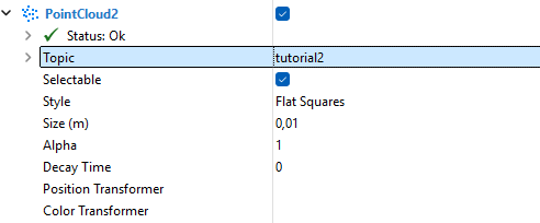
Adjust visualization settings to make points easier to see (e.g. Frame Rate: 60, Style: Points, Decay time: 0,2)
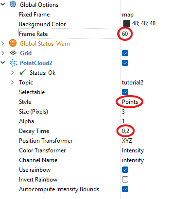
Now, if scene 2 of the tutorial is active and both programs are launched using the same ROS domain ID, the points produced by the lidar instance in agxViewer will be displayed in
RViz.
33.3.1.3. Troubleshooting
If messages are missed, or the first couple of messages are missed, it may be of use to check the QOS settings used.
By default the QOS settings are the same as in ROS2, i.e. RELIABILITY “reliable”, DURABILITY “volatile”, HISTORY “keep last” and history depth 10.
More details on these settings can be seen (here).
If no communication between a built in agxROS2::Publisher and a built in agxROS2::Subscriber can be established it is possible that it is blocked by a firewall on the computer. Check the firewall settings and unblock the process in case it has been blocked.
If no communication between a built in agxROS2::Publisher/Subscriber and an external ROS2 node running on a complete ROS2 installation can be established, ensure that the same version of ROS2 is used.
The built in ROS2 support in AGX Dynamics targets ROS2 Humble.
If this does not solve the problem, ensure that the DDS implementation Fast-DDS is used in the ROS2 installation.
This can be forced by setting the environment variable RMW_IMPLEMENTATION=rmw_fastrtps_cpp. See the (ROS2 documentation) for details.
Also check the firewall settings if necessary.
If the creation of a agxROS2::Publisher or agxROS2::Subscriber hangs forever it is possible a seemingly rare bug in Fast-DDS is the culprit.
This seems to happen when creating a DDS Participant (which is done automatically by AGX Dynamcis) on Windows on rare occations.
The underlying reason why this can happen is not known, but a manual workaround is to do the following:
1. Turn off any process using ROS2.
2. Manually remove all files in C:\ProgramData\eprosima\fastrtps_interprocess (replace drive-letter if applicable).
33.3.1.4. Using custom types
There is some built in support for sending custom data types via ROS2.
This is done using the AnyMessageBuilder and AnyMessageParser.
The AnyMessageBuilder can serialize and deserialize several common built in primitive types to an agxMsgs::Any message.
This message can then be sent on any Topic, received and deserialized using the AnyMessageParser.
The agx_msgs::Any message type as well as AnyMessageBuilder and AnyMessageParser are also avaiable open-source on GitHub so that these can be used on machines that does not have AGX Dynamics or installed.
Below is a small example of how this can be used.
#include <agxROS2/AnyMessageBuilder.h>
#include <agxROS2/AnyMessageParser.h>
#include <agxROS2/Publisher.h>
#include <agxROS2/Subscriber.h>

struct MyStruct
{
  std::string myString;
  std::vector<int64_t> myInts;
  float myFloat{ 0.f };
};

int main()
{
  // Custom struct that we will send via ROS2.
  MyStruct sendStruct;
  sendStruct.myString = "We are all star stuff";
  sendStruct.myInts = { 42, 13, -999 };
  sendStruct.myFloat = 2.71828f;

  // Create Publisher and Subscriber with specific Topic.
  agxROS2::agxMsgs::PublisherAny pub("any_msg");
  agxROS2::agxMsgs::SubscriberAny sub("any_msg");

  // Serialize the custom struct type.
  agxROS2::AnyMessageBuilder builder;
  builder
    .beginMessage()
    .writeString(sendStruct.myString)
    .writeInt64Sequence(sendStruct.myInts)
    .writeFloat32(sendStruct.myFloat);

  // Send the message.
  pub.sendMessage(builder.getMessage());

  // Try to receive the message.
  agxROS2::agxMsgs::Any msgReceive;
  if (!sub.receiveMessage(msgReceive))
  {
    std::cout << "Dit not receive a message.\n";
    return 1;
  }

  // De-serialize the message and read back the custom struct that was received.
  MyStruct receiveStruct;
  agxROS2::AnyMessageParser parser;
  parser.beginParse();
  receiveStruct.myString = parser.readString(msgReceive);
  receiveStruct.myInts = parser.readInt64Sequence(msgReceive);
  receiveStruct.myFloat = parser.readFloat32(msgReceive);

  // receiveStruct now contains the data that was sent by the publisher.

  return 0;
}
Another example of this is available in the tutorial tutorials/agxOSG/tutorial_ros2.cpp.
33.3.2. Pre-built ROS2 installation
The pre-built ROS2 installation is available for Windows only. It can be installed through the AGX Dynamics installer. At the end of the AGX Dynamics installation, there is a checkbox to download and unzip a pre-built ROS2. It can also be downloaded manually from (here).
Un-zip it and place it in C:\opt such that the path to local_setup.bat is C:\opt\ros2-algoryx\install\local_setup.bat.
The placement of the ROS2 installation must match exactly this.
The pre-built ROS2 installation is of version ROS2 Humble.
To be able to build custom ROS2 packages, CMake and Visual Studio must be installed manually on the computer.
There is no specific AGX Dynamcis integration when using this alternative, but it is possible to use AGX Dynamics and a ROS2 installation in the same Python environment. Here, a simple ROS2 Publisher class and a ROS2 Subscriber class is added to an AGX Python script.
# Include the necessary ROS2 modules.
import rclpy
from rclpy.node import Node
from std_msgs.msg import Float32

# ROS2 publisher class.
class RosPublisher(Node):
  def __init__(self, node_name, topic_name):
    super().__init__(node_name)

    self.publisher = self.create_publisher(Float32, topic_name, 1)

  # Publish a ROS2 message.
  def send_data(self, data):
    msg = Float32()
    msg.data = data
    self.publisher.publish(msg)

# ROS2 subscriber class.
class RosSubscriber(Node):
  def __init__(self, node_name):
    super().__init__(node_name)

  # Note: the callback function must have an input parameter for the message.
  def register_callback(self, topic, callback_function):
    self.create_subscription(
      Float32,
      topic,
      callback_function,
      1)
33.4. URDF
AGX Dynamics provides a URDF reader that takes a URDF file and returns an AGX Dynamics representation of the model.
33.4.1. UrdfReader class
The agxModel::UrdfReader class has a static read method for reading urdf files and returning an agxSDK::Assembly object with all the robot parts (bodies, geometries and constraints).
The behavior of the read method can be controlled using the agxModel::UrdfReader::Settings class. See the examples below for more information.
33.4.2. Examples
Below are two simple examples of how to read a URDF model and access one of its joints, both in C++
and Python. Also, instructions for running the URDF Panda ROS2 Python example is described below.
33.4.2.1. C++ example
Read a URDF model and access one of its joints.
// Absolute path to the URDF file.
agx::String urdfFile = "absolute/path/model_package/description/model.urdf";

// (Optional) Absolute path to the URDF package path pointing to the 'package://'
// part of any filename attribute in the URDF file if existing.
agx::String urdfPackagePath = "absolute/path/model_package";

// (Optional) Initial joint positions. Must match in length the total number of
// revolute, continous and prismatic joints in the model.
agx::RealVector initJointPos {agx::PI/2.0, -agx::PI/4.0, 0.0, 0.0, 0.0, 0.0};

agxModel::UrdfReader::Settings settings;

// Determines if the base link of the URDF model should be attached to the
// world or not.
// Default is false.
settings.attachToWorld = true;

// If true the collision between linked/constrained bodies will be disabled.
// Default is false.
settings.disableLinkedBodies = true;

// If true, any link missing the <inertial></inertial> element will recieve
// a negnegligible mass and will be treated as a kinematic link
// and will be merged with its parent. According to http://wiki.ros.org/urdf/XML/link
// If false, the body will get its mass properties calculated from the shape/volume/density.
// Default is True.
settings.mergeKinematicLink = true;

// Read the URDF.
agxSDK::AssemblyRef model =
  agxModel::UrdfReader::read(urdfFile,
                             urdfPackagePath,
                             &initJointPos,
                             settings);

// Add the model to the agxSDK::Simulation.
simulation->add(model);

// Access one of the joints in the model and set wanted speed for it. The name of the constraint
// corresponds to the name of the joint in the URDF file.
agx::Constraint1DOF* joint1 = model->getConstraint1DOF("joint_name");
joint1->getMotor1D()->setEnable(true);
joint1->getMotor1D()->setSpeed(0.5);
33.4.2.2. Python example
Read a URDF model and access one of its joints.
# Absolute path to the URDF file.
urdfFile = "absolute/path/model_package/description/model.urdf"

# (Optional) Absolute path to the URDF package path pointing to the 'package://'
# part of any filename attribute in the URDF file if existing.
urdfPackagePath = "absolute/path/model_package"

# (Optional) Initial joint positions. Must match in length the total number of
# revolute, continous and prismatic joints in the model.
initJointPos = agx.RealVector()
initJointPos.append(agx.PI/2.0)
initJointPos.append(-agx.PI/4.0)
for i in range(0, 4):
  initJointPos.append(0.0)

# Determines if the base link of the URDF model should be fixed to the
# world or not. Default is false.
fixToWorld = True

# If true the collision between linked/constrained bodies will be disabled.
# Default is false.
disableLinkedBodies = True

# If true, any link missing the <inertial></inertial> key will be treated
# as a kinematic link and will be merged with its parent. According to http://wiki.ros.org/urdf/XML/link
# If false, the body will get its mass properties calculated from the shape/volume/density.
# Default is True.
mergeKinematicLink = True

settings = agxModel.UrdfReaderSettings(fixToWorld, disableLinkedBodies, mergeKinematicLink)

# Read the URDF.
model = agxModel.UrdfReader.read(urdfFile, urdfPackagePath, initJointPos, settings)

# Add the model to the agxSDK.Simulation. Notice the .get() which is needed since model
# is an agxSDK.AssemblyRef.
sim.add(model.get())

# Access one of the joints in the model and set wanted speed for it. The name of the constraint
# corresponds to the name of the joint in the URDF file.
joint1 = model.getConstraint1DOF("joint_name")
joint1.getMotor1D().setEnable(True)
joint1.getMotor1D().setSpeed(0.5)
33.4.2.3. ROS2 URDF Panda example
Start the URDF Panda robot simulation
Simply double-click the urdf_panda_ros2.agxPy located in Algoryx/AGX-version/data/python/ROS2.
Start the URDF Panda ROS2 controller
Open a new “AGX Dynamics Command Line”.
In the AGX command prompt, cd to the AGX ROS2 examples directory, e.g:
cd Algoryx/AGX-version/data/python/ROS2
Run the URDF Panda ROS2 controller script by calling python, i.e:
python urdf_panda_ros2_controller.py
33.4.3. Supported features overview
Below is an overview of the URDF features. Those marked with ‘✓’ are supported by the URDF reader and those marked with ‘☓’ are not.
robot ✓
│   name ✓
│
└───link ✓
│   │   name ✓
│   │
│   └───inertial ✓
│   │   │
│   │   └───origin ✓
│   │   │      xyz ✓
│   │   │      rpy ✓
│   │   │
│   │   └───mass ✓
│   │   │      value ✓
│   │   │
│   │   └───intertia ✓
│   │          ixx - izz ✓
│   │
│   └───visual ✓
│   │   │   name ✓
│   │   │
│   │   └───origin ✓
│   │   │      xyz ✓
│   │   │      rpy ✓
│   │   │
│   │   └───geometry ✓
│   │   │   │
│   │   │   └───box ✓
│   │   │   │      size ✓
│   │   │   │
│   │   │   └───cylinder ✓
│   │   │   │      radius ✓
│   │   │   │      length ✓
│   │   │   │
│   │   │   └───sphere ✓
│   │   │   │      radius ✓
│   │   │   │
│   │   │   └───mesh ✓
│   │   │          filename ✓
│   │   │          scale ✓
│   │   │
│   │   └───material ✓
│   │       │   name ✓
│   │       │
│   │       └───color ✓
│   │       │      rgba ✓
│   │       │
│   │       └───texture ✓
│   │
│   └───collision ✓
│       │   name ✓
│       │
│       └───origin ✓
│       │      xyz ✓
│       │      rpy ✓
│       │
│       └───geometry ✓
│              (see geometry under 'visual' above)
│
└───joint ✓
│   │   name ✓
│   │   type: revolute ✓
│   │   type: continuous ✓
│   │   type: prismatic ✓
│   │   type: fixed ✓
│   │   type: floating ✓
│   │   type: planar ✓
│   │
│   └───parent ✓
│   │      link ✓
│   │
│   └───child ✓
│   │      link ✓
│   │
│   └───axis ✓
│   │      xyz ✓
│   │
│   └───calibration ☓
│   │
│   └───dynamics ✓
│   │      damping ☓
│   │      friction ✓
│   │
│   └───limit ✓
│   │      lower ✓
│   │      upper ✓
│   │      effort ✓
│   │      velocity ☓
│   │
│   └───mimic ✓
│   │      multiplier ✓
│   │      offset ✓
│   │
│   └───safety_controller ☓
│
└───transmission ☓
│
└───gazebo ☓
│
└───sensor ☓
│
└───model_state ☓
33.4.4. AGX Dynamics representation
Below is a detailed description of the how the URDF features are represented by AGX Dynamics.
33.4.4.1. <robot>
The root element robot is represented by an agxSDK::Assembly. The name of the agxSDK::Assembly
is set to the required name attribute.
33.4.4.2. <link>
Each link is represented by an agx::RigidBody. The name of the agx::RigidBody is set to
the required name attribute.
33.4.4.2.1. <inertial>
The optional inertial element determines the mass and intertial properties of the agx::RigidBody. If no
inertial element exist for a link, then AGX Dynamis will automatically calculate the mass properties based on
all visual elements. The reason for using the visual elements is that it in most cases will have a more correct volumetric representation of the robot compared to the collide elements.
The behaviour of the reader can be controlled using the UrdfReader::Settings class.
33.4.4.2.1.1. <origin>
The optional origin element determines the center of mass of the agx::RigidBody. If not specified
(but inertial is), then identity position and orientation is used.
33.4.4.2.1.2. <mass>
The mass element determines the mass of the agx::RigidBody. This is a required attribute for any
inertial element.
33.4.4.2.1.3. <inertia>
The inertia element determines the inertia of the agx::RigidBody with respect to its center of mass.
This is a required attribute for any inertial element.
33.4.4.2.2. <visual>
Each visual element is represented by a agxCollide::Geometry with collision disabled. The name of
the agxCollide::Geometry is set to the optional name attribute if it is specified.
33.4.4.2.2.1. <origin>
The optional origin element determines the position and orientation of the agxCollide::Geometry with respect to the owning
agx::RigidBody. Identity position and orientation is used if not specified.
33.4.4.2.2.2. <geometry>
The required geometry element is represented by an agxCollide::Shape where box,
cylinder and sphere are represented by the corresponding AGX Dynamics primitive shapes. Any mesh
element is represented by a agxCollide::Trimesh.
33.4.4.2.2.3. <material>
The optional material element is represented by a agxCollide::RenderMaterial. Note that if a texture is
specified, the texture information will be lost if a serialize/deserialize cycle of the scene is done and
the underlying texture resouce (pointed to by the filename attribute) is moved or removed.
33.4.4.2.3. <collision>
Each collision element is handled similarly as a visual element but has collision enabled.
Any agxCollide::Geometry representing a collision element is given empty agxCollide::RenderData
meaning it will not be rendered to the screen if not debug rendering is active. Since it is not
rendered, any material element inside a collision element is ignored. Note that a collision
element does not affect the automatically calculated mass properties of a agx::RigidBody representing
the parent link in the case where no inertial element exists. Only the visual elements are
used in the calculation for that case.
33.4.4.2.4. <joint>
Each joint element is represented by an agx::Constraint. The name of the agx::Constraint
is set to the required name attribute. Any revolute joint is represented by an agx::Hinge with the
secondary constraint agx::RangeController active. Any continuous joint is represented by an
agx::Hinge. Any prismatic joint is represented by an agx::Prismatic with the secondary
constraint agx::RangeController active. Any fixed joint is represented by an agx::LockJoint.
Any floating joint is ignored since free body movement is the default behaviour of any agx::RigidBody.
Any planar joint is represented by an agx::PlaneJoint.
33.4.4.2.4.1. <origin>
The optional origin element specifies the position and orientation of the child agx::RigidBody
representing the child link with respect to the parent agx::RigidBody representing the parent
link. If not specified identity position and orientation is used.
33.4.4.2.4.2. <parent>
The required link attribute of the required parent element specifies the name of the parent
agx::RigidBody that is attached to the agx::Constraint representing the joint.
33.4.4.2.4.3. <child>
The required link attribute of the required child element specifies the name of the child
agx::RigidBody that is attached to the agx::Constraint representing the joint.
33.4.4.2.4.4. <axis>
The optional axis element determines the axis of rotation for any agx::Hinge representing
a revolute or continuous joint, or the axis of translation for any agx::Prismatic
representing a prismatic joint. If not specified, then [1, 0, 0] is used.
33.4.4.2.4.5. <calibration>
Not supported and will be ignored.
33.4.4.2.4.6. <dynamics>
The optional dynamics element determines the dynamic behaviour of the agx::Constraint representing a
joint. If not specified the default AGX Dynamics parameters are used for the agx::Constraint.
Not supported and will be ignored. Note that it is possible to manually set the damping for any DOF for a
agx::Constraint representing a joint. This can be done by accessing the agx::Constraint
from the returned agxSDK::Assembly followed by calling the function agx::Constraint::setDamping(…).
The optional friction attribute specifies the static friction of the joint in Newtons. This
corresponds to a force range of the secondary constraint agx::FrictionController of the
agx::Constraint and is applied as such.
If the friction attribute is not specified, the default AGX Dynamics friction is used.
33.4.4.2.4.7. <limit>
The limit element specifies the upper and lower bounds of of the joint both in terms of rotational/translational freedom and in maximal force/torque. The limit element is supported only for revolute and prismatic joint’s and for those it is also a required element.
The lower and upper attributes are represented as the lower and upper range of the secondary
constraint agx::RangeController and are applied as such. If not specified, then 0 is used for
both attributes.
The required effort attribute specifies the maximum force/torque of the agx::Constraint’s secondary
constraints: agx::RangeController, agx::LockController and agx::TargetSpeedController.
The velocity attribute is not supported and will be ignored.
33.4.4.2.4.8. <mimic>
The optional mimic element makes it possible to configure an agx::Constraint representing
the joint in such a way that it will move in accordance with another agx::Constraint.
Internally any mimic element is represented as a agxPowerLine::PowerLine with a number of
agxPowerLine::Connector’s together with an agxDriveTrain::Gear configured to give this
behaviour. The mimic feature is supported for revolute, continuous and prismatic joint’s.
Having a revolute or continuous joint mimic a prismatic joint or vice versa is not supported,
but having a revolute joint mimic a continuous joint or vice versa is.
The optional multiplier attribute corresponds to a gear ratio of the agxDriveTrain::Gear that
is part of the agxPowerLine::PowerLine representing the mimic element.
If not specified the value 1 is used.
The optional offset attribute will add an initial rotational or translational offset to the
agx::Constraint representing the joint with the mimic element. If an initial joint
value is set using the joints parameter when calling the agxModel::UrdfReader::read() function,
the offset attribute will be added to this initial joint value.
33.4.4.2.4.9. <safety_controller>
Not supported and will be ignored.
33.4.4.3. <transmission>
Not supported and will be ignored.
33.4.4.4. <gazebo>
Not supported and will be ignored.
33.4.4.5. <sensor>
Not supported and will be ignored.
33.4.4.6. <model_state>
Not supported and will be ignored.