31. Performance¶

This section will describe different methods and techniques that can be applied to simulations in AGX to increase the runtime performance.

Some methods are described in other sections:

Use multiple threads, see Section 31.5
Use agxSDK::MergeSplitHandler (AMOR), see Section 32.2
Use agx::MergedBody (Section 32.1)

31.1. Contact viscosity¶

If you are using the DIRECT solver for contact friction (see Section 11.16.4) you can sometimes achieve improved performance by increasing the viscosity in the contact material.

31.2. Contact Warmstarting¶

In Section 11, friction models were explained. Which friction model(s) that are in use can affect the runtime performance in a large way. Scale-box-friction for example provides a more realistic model than box-friction at the expense of a higher runtime cost due to more numeric work in the solver.

The cost of scale-box-friction can in some scenarios be reduced by enabling contact warmstarting via

agx::DynamicsSystem::setEnableContactWarmstarting( bool enable )

This feature will map internal solver states from the previous timestep to the current one by matching the previous contact point positions and normals to the current ones. The solver is then warmstarted and have the possibility to reduce the amount of work needed to solve the system.

When the default friction model is used and no special handling is setup via contact materials, enabling contact warmstarting will just add overhead since extra steps are enabled that checks if data should be cached and if contact points should be matched from timestep to timestep.

Attention

The internal states used for warmstarting contacts are not part of the data that is serialized. Creating a simulation and simulating for e.g. 10 seconds can have slightly different trajectories compared to a different simulation with the same initial state that was simulated for 5 seconds, stored, restored and then simulated an additional 5 seconds.

31.3. Using Iterative contact solver¶

In Section 3.4 the different solvers available in AGX Dynamics where described. If you have performance challenges and you are willing to sacrifice precision for performance, the Iterative solver can be used for solving contact friction. As described in Section 11.16.4 we can control solve type for each ContactMaterial by creating a Friction model.

Assume for example you have a scenario where you are using a machine (wheel loader, excavator) and you want to interact with many (hundreds) of rocks, the performance might be an issue when using the default (SPLIT) contact model.

Assume you have a Material for the rocks and you want to use the ITERATIVE solve model for anytime two rocks interact:

// Create a material for the rocks
// Then (not shown) you need to assign each "rock" geometry the new material
agx::MaterialRef rockMaterial = new agx::Material("Rock")

// Get (or create if not already created) the ContactMaterial for the Rock/Rock material interaction
agx::ContactMaterialRef rock_rock_cm = simulation->getMaterialManager()->getOrCreateContactMaterial(rockMaterial, rockMaterial);

// Create a new FrictionModel, we will use the friction model which is default in AGX:
agx::FrictionModelRef fm = new agx::IterativeProjectedConeFriction();
fm->setSolveType( agx::FrictionModel::ITERATIVE );

// Assign the friction model to the contact material
rock_rock_cm->setFrictionModel(fm);

By using the code above, AGX will now use the fast ITERATIVE solver for any contacts between two geometries using the “Rock” material.

Section 9.8 show an example in how to combine the ITERATIVE and the DIRECT solver in the same scene.

31.4. AGX Sabre¶

The overview in Table 3.1 mentioned that agxSabre contains a sparse matrix solver. The sparse matrix is blocked so that BLAS-like kernels can be used to achieve better performance.

By default AGX will select which kernels to use and this default value should be left alone for best performance. But if the user really wants to, the setting can also be changed by the function

bool agxSabre::SabreKernels::setPreferredVectorInstructionSet( bitmask )

AGX Sabre will check which hardware features that are supported during library initialization. Unsupported features in the input value to setPreferredVectorInstructionSet will then be masked away.

The bit in the instruction set bitmask which has the largest effect is AVX2_BIT which enables fused-multiply-add instructions.

Which kernels to use can also be configured via the environment variable AGXSABRE_KERNELS and that variable accepts the same values as setPreferredVectorInstructionSet. For verification, the environment variable AGXSABRE_VERBOSE_KERNELS can be set to recieve a printout on stdout such as [agxSabre] Detected "GenuineIntel" CPU with HW features 7, preferred features set to 7 to see how the hardware was identified. Additionally, if AGXSABRE_KERNELS is also set, two lines will be displayed, e.g.:

[agxSabre] Environment set preferred vector instruction set to 15
[agxSabre] Detected "AuthenticAMD" CPU with HW features 15, preferred features set to 15

31.5. Parallelization¶

In Fig. 10.2 we could see that some of the items were marked with an asterisk (*). This indicates that the subtask is a potential target for parallelization. In this section the various tasks will be dissected in more detail.

AGX is built upon the notion of tasks. A task can depend on other tasks and can also have sub-tasks. A Task which does not depend on other tasks can run in parallel with other tasks.

For example the class DynamicsSystem is built upon several tasks and subtasks. Such as “UpdateWorldMassAndInertia”, “IntegrateVelocity”, etc. Many of these tasks will split up the work and execute in parallel. Another important feature of AGX is that all of the critical data for rigid bodies, shapes etc. are stored in buffers. These buffers are memory allocation blocks, aligned in memory appropriately for SSE optimization. Also, the memory can be made available for other implementation platforms such as OpenCL or CUDA. The executional part of a task is called a kernel. It can have several implementations, SSE, non-SSE, OpenCL, OpenGL etc. Which type of implementation that is needed, is selected when the task/kernel is initialized. A kernel is a small executional unit which operates on indata and supplies the result as out-data. It operates directly on the buffers for the fastest possible data access. This schema makes it possible to have some kernels executing on the graphics cards (for example OpenCL kernels), and some on the CPU.

31.5.1. Threads¶

In AGX there is a pool of threads used for all threaded jobs. The size of this pool is controlled with the call:

agx::setNumThreads( int n );

A negative value for n means that one thread is created per Core/CPU. The default value is 1. All parallelizable tasks are job-oriented. All jobs are put into a queue and scheduled for execution.

31.5.1.1. Executing AGX in threads¶

AGX creates and manages its own threads in a thread pool. However, to use the AGX API you need to be aware of a few things:

Any thread that calls the AGX API need to be registered as an AGX thread. This is because various resources need to be available for each thread. To promote a thread to be an AGX Thread call:

agx::Thread::registerAsAgxThread();

To unregister a thread, call:

agx::Thread::unregisterAsAgxThread();

Callbacks from AGX such as contact events (10.4.3) or from event listeners (10.4.6) will always be done to the main thread for an agxSDK::Simulation. This is the thread that created the agxSDK::Simulation object. To make a thread the main thread for a simulation call (after a call to registerAsAgxThread()):

simulation->setMainWorkThread( agx::Thread::getCurrentThread() );

For an example of this, see tutorial_threads.cpp

31.5.2. Parallel tasks¶

Table 20 below; show some of the tasks which are parallelizable. These tasks will however not run in parallel to each other, as they depend on data from the previous task. Compare to the time line for the call to Simulation::stepForward() (Fig. 10.2).

Table 31.1 Parallelizable tasks¶
Name	Description	Belongs to
NarrowPhase	Calculates contact data between two overlapping Geometries.	agxCollide::Space
Update bounding volumes	Update bounding volumes for geometries.	agxCollide::Space
ApplyGravity	Add gravitational force to bodies.	agx::DynamicsSystem
Solver	Solve the constraint system.	agx::DynamicsSystem
IntegratePositions	Integrate transformation and calculate acceleration.	agx::DynamicsSystem
IntegrateVelocity	Integrate Velocity	agx::DynamicsSystem
UpdateWorldMassAndInertia	Will calculate various items needed for the solver.	agx::DynamicsSystem

The Solver stage is only parallelizable if the partitioner can create disjoint groups of bodies which can be solved independently from each other.

31.5.2.1. NarrowPhase¶

This task will be given a list of overlapping bounding volumes (from the broad phase) calculate the exact contact data for two possibly overlapping geometries. This is a trivially parallelizable task, as there are no data dependency between the different overlapping geometries.

31.5.2.2. Update bounding volumes¶

This task will update the current bounding volume for a geometry (including its shape transformation and size). Depending on the frame hierarchy, this task can occupy quite some time for a large number of geometries. There are no data dependencies between the geometries. It can therefore be parallelized.

31.5.2.3. Partitioner¶

Based upon the connectivity in the whole dynamics system, the partitioner can split the system into independent sub-systems.

Two bodies are connected if there is a constraint between them. Constraints including contacts can create large trees of interconnected bodies.

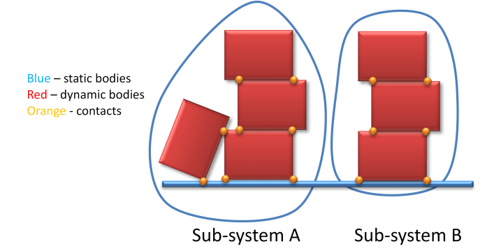
Fig. 31.1 Two separate subsystems.¶

In the figure above, two separate systems can be identified which can be solved independently from each other, hence the above system would gain if the solver would run the two systems in one thread each. As soon as there is a connection (through a constraint/contact) between two systems, they are merged. Kinematic bodies will analogous to static bodies split a system into two parts allowing for parallelization.

31.6. Contact reduction¶

By using contact reduction, the number of contact points later submitted to the solver as contact constraint can be heavily reduced, hence improving performance.

31.6.1. Motivation¶

Assuming that a rigid body has one or several geometries associated, when these geometries collide with the geometries from another rigid body, contact points will be generated. Given a complicated geometry or shape, or many overlapping geometries, potentially a large number of contact points will be created. Each contact point will later lead to a contact constraint which must be handled by the solver. Since frictional contacts are relatively expensive to solve, a large number of contact points will have a negative effect on performance. Also, in some cases too many contacts can lead to an over-determined system and cause the simulation to deliver bad results.

For example: a box (primitive) on a plane only needs 3-4 contacts to stand stable whereas in a different scenario where the box is a tesselated mesh resting on a tesselated plane we can easily get hundreds of contact points.

31.6.2. Technical details¶

The reduction is done by the class agxCollide::ContactReducer, where contact points are reduced by a 6-dimensional binning algorithm in [nxp, n]-space. Here, n is the contact normal and p the contact point relative to a reference point (e.g. one body’s center of mass, or the world origin).

In the overall physics pipeline, contacts can get reduced in two separate stages:

Directly in the narrow phase stage, contact reduction is done on each geometry-geometry interaction (can be controlled, see below). Contact points that are reduced get removed immediately.
After collision detection and before stepping the Dynamics system (i.e. PRE in a StepEventListener), contact reduction is done on some rigidbody-rigidbody interactions (can be controlled, see below).

The contact reduction within the physics pipeline can be controlled in three ways:

By setting the reduction mode: ContactReductionMode. Either no reduction, or per geometry overlap, or per geometry overlap AND per rigid body overlap.
By setting the bin resolution \(b\), number of bins per dimension. Given a bin resolution of \(b\), this could lead to \(b^6\) contacts being left after reduction in worst case. Average case is about \(b^2\). The bin resolution can be set differently for geometry overlaps and rigid body overlaps. A high value will keep more contacts, lower will result in more aggressive reduction. Commonly a value of 2-3 will give good results. Default is 3. Values from 1 to 10 are valid.
By setting the threshold for doing contact reduction. In order to not waste time on doing contact reduction for contacts with small numbers of contact points, contact reduction is only done on contacts which exceed a certain number of contact points. This threshold can be set separately for geometry-geometry-overlaps and rigidbody-rididbody-overlaps.

It is possible to call agxCollide::ContactReducer::reduce manually. One motivation for this might be if you want to analyze all contact points before sending them to the solver. This can be done by:

setting the reduction mode to REDUCE_NONE for a contact material,
and then in a ContactEventListener:

analyzing the contacts as desired

making a manual call to agxCollide::ContactReducer::reduce to reduce the number of contacts that reaches the solver

Note

Modifying contacts might interfere with other ContactEventListeners listening to the same contact! Currently, the only way to modify contact points that should reach the solver is via a ContactEventListener.

31.6.3. ReductionMode¶

AGX has two steps where contacts are reduced:

For a pair of overlapping geometries (with potentially several shapes)
For a pair of overlapping rigid bodies (with potentially several geometries).

By default, AGX does one contact reduction pass between each pair of overlapping geometries.

This behavior can be changed to one of the three modes:

/// Specifies the mode for contact reduction
enum ContactReductionMode {
  REDUCE_NONE,               /**< No contact reduction enabled */
  REDUCE_GEOMETRY,           /**< Default: Reduce contacts between geometries */
  REDUCE_ALL                 /**< Two step reduction: first between geometries, and then between rigid bodies */
};

The contact reduction mode can be set per contact material. An example:

// We want to reduce contacts not only between each geometry, but between body and other body

// Assume we have a body and five geometries, each with e.g. one or more trimesh shapes.
rigidBody->add( geometry1 );
rigidBody->add( geometry2 );
rigidBody->add( geometry3 );
rigidBody->add( geometry4 );
rigidBody->add( geometry5 );

// Assign a material to the geometries
geometry1->setMaterial( material1 );
geometry2->setmaterial( material1 );

// Assume we also have another body which we also assign a material to
otherBody->add( otherGeometry );
otherGeometry->setMaterial( material2 );

// Create a new contact material
agx::ContactMaterialRef cm = simulation->getMaterialManager()->getOrCreateContactMaterial(material1, material2);

// Set contact reduction mode to REDUCE_ALL - now, contacts between rigidBody and otherBody
// get reduced together, not only each contact by itself.
cm->setContactReductionMode( agx::ContactMaterial::REDUCE_ALL );

Note that REDUCE_ALL is not the default for a reason:

Often, bodies are assigned different geometries because one would like to set different materials on these geometries, resulting in different physical behavior (e.g. vary friction, Young’s modulus, …).

Contact reduction with REDUCE_ALL does not take these differences into account, but reduces over all contact points. However, each contact point will remain in the GeometryContact it belongs to, and only GeometryContacts with a contact material with REDUCE_ALL set will be reduced upon.

All geometries without a rigid body will be treated as belonging to the same one when doing contact reduction between rigid bodies. If you want to avoid geometry contacts from several geometries without rigid bodies to end up in the same reduction, move these geometries into separate (static) rigid bodies.

31.6.3.1. Bin resolution¶

The bin resolution gives the number of bins per dimension. Given a bin resolution of n, this could lead to n^6 contacts in worst case, where the average case is about c*n^2 (common contact region, like in convex overlaps).

The bin resolution can be set differently for geometry overlaps and rigid body overlaps, as well as for manual contact reduction.

In the general case, a bin resolution of between 1 and 10 is allowed, where typical values are 2 or 3.

Below is a more detailed description.

31.6.3.1.1. Geometry overlaps¶

The bin resolution for contact reduction for rigid body overlaps can only be given for the whole simulation by setting the value like in this example:

// Set contact reduction bin size to 3 for simulation (rigid body overlaps).
sim->setContactReductionBinResolution( 3 );

The bin resolution for contact reduction for geometry overlaps can be set per contact material:

// Create a new contact material
agx::ContactMaterialRef cm = simulation->getMaterialManager()->getOrCreateContactMaterial(material1, material2);

// Set contact reduction bin size to 3 for contact material (all geometry overlaps with this contact material).
cm->setContactReductionBinResolution( 3 );

If the bin resolution is set to zero (not allowed in other contexts, see above) in the contact material or if no contact material is used, a fallback value from agxCollide::Space is used which can be specified like in this example:

// Set contact reduction bin size to 3 for space (fallback value for geometry overlaps).
agxCollide:;SpaceRef = sim->getSpace();
space->setContactReductionBinResolution( 3 );

31.6.3.1.2. Rigid body overlaps¶

The bin resolution for contact reduction for rigid body overlaps can only be given for the whole simulation by setting the value like in this example:

// Set contact reduction bin size to 3 for simulation (rigid body overlaps).
sim->setContactReductionBinResolution( 3 );

31.6.3.1.3. Manual contact reduction¶

The bin resolution for manual contact reduction can be given in the reduce-call to contact reducer (a static method):

// Set contact reduction bin size to 3 for simulation (rigid body overlaps).
size_t binResolution = 3;
agxCollide::ContactReducer::reduce(contactPoints, binResolution);

31.6.3.2. ContactReductionThreshold¶

The contact reduction between overlapping geometries is enabled by default (otherwise dependent on the material’s reduction mode, see chapter above) and will be activated when the number of contact points between two geometries is larger than a specified threshold. This threshold is set globally in agxCollide::Space (since space is responsible for geometries):

agxCollide::SpaceRef space = new agxCollide::Space();
// More than 10 contact points will trigger contact reduction
space-> setContactReductionThreshold( 10 );

The additional contact reduction between overlapping rigid bodies is disabled by default (otherwise dependent on the material’s reduction mode, see ReductionMode) and will be activated when the number of contact points between two rigid bodies is larger than a specified threshold. This threshold is set globally in agxSDK::Simulation:

agxSDK::SimulationRef sim = new agxSDK::Simulation();
// More than 10 contact points will trigger contact reduction
sim-> setContactReductionThreshold( 10 );