12. Constraints¶

A Constraint will define a geometrical relationship between one rigid body relative to the world, or two or more rigid bodies relative to each other, that should be met under certain conditions. Each constraint is built upon elementary constraints, which define the geometrical relationship. Acting upon these elementary constraints can be secondary order constraints, motors, limits or locks.

Example of how to use the constraint API is showcased in the tutorials/tutorial_tutorial5.cpp

One important thing to keep in mind when constructing systems with constraints is that:

Attention

Always position/rotate the rigid bodies involved in a constrained system before attaching them to a constraint.

Available constraints in the current AGX version are:

Table 12.1 Available constraints¶
CONSTRAINT NAME	DESCRIPTION
BallJoint	Ball and socket joint
DistanceJoint	Restore distance between two specified points on bodies.
Hinge	Allow rotation around one specified axis (revolve)
UniversalJoint	Transmission joint.
LockJoint	Removes all degrees of freedom between two bodies, keep the locked together.
Prismatic	Allows translation along one axis (slide)
PlaneJoint	Reduce translation movement to a plane
CylindricalJoint	Hinge and Prismatic combined
AngularLockJoint	Reduces all rotational DOF between two bodies.
SplineJoint	Allows movement along a spline. Related to CylindricalJoint.
WheelJoint	Allows for rotation around two axes (wheel, steering) and movement along one (steering for suspension).

Some of the constraints have one additional version which includes support for having slack in the joint to model a non-ideal joint. These are:

Table 12.2 Available constraints with slack¶
CONSTRAINT NAME
SlackCylindricalJoint
SlackHingeJoint
SlackLockJoint
SlackPrismaticJoint

Slack joints can be used to model a system with a specified gap. Let’s say you are modeling a robot with a tool. The tool is attached to the robot arm, but the tool has a few millimeters slack in translation. Modeling this using collision detection can be complicated and resource demanding. Small features usually mean you have to use shorter time steps. With a slack joint, this gap can be modelled using a constraint. This allows for better performance and much more reliable result.

Each slack joint has slack range parameters which can be controlled. Depending on which constraint is being used, there are different number of degrees of freedom available for the slack modeling. For example, the SlackLockJoint has 6 DOF for slack modelling, whereas the SlackPrismaticJoint only has 5 (the fifth is the free DOF controlled using motors/lock/range).

The slack can be both positional (meter) and rotational (radians). If the slack feature is not needed, then it is better to use the ordinary version of the constraint. The reason for this is that the ordinary version uses half the number of equations compared to the slack version and will therefore be faster for the solver to handle.

Note

Currently the slack joints only has one argument for the rotational slack. This means that the rotational slack is applied to all rotational degrees of freedoms.

12.1. Elementary constraints¶

Elementary constraints are constraints that ordinary, more complex constraints are based upon. These elementary constraints are:

Table 12.3 Elementary constraints¶
NAME	DESCRIPTION
Dot-1	Given two vectors v₁ and v₂, this constraint will retain v₁ · v₂ = 0.
Dot-2	Given a separation vector d^ij between body i and j and and body fixed vector aⁱ, this constraint will retain d^ij · aⁱ = 0.
Spherical	This is a 3D constraint which computes xⁱ + pⁱ - x^j – p^j = 0, where x is a body fixed vector and p the position of that vector.
Distance	Given two positions pⁱ and p^j, this constraint will retain \| pⁱ – p^j \| = l_o, where l₀ is some constant.
QuatLock	Locks all rotational degrees of freedom between two bodies.

For example, a hinge is a composite of two Dot-1 and one Spherical elementary constraint.

12.1.1. Converting spring constant and damping¶

In the agxUtil namespace there are functions for converting from the spring constant and damping to AGX regularization parameters:

Converting from a spring constant to compliance: compliance = 1/springConstant:

// Convert from a spring constant to compliance
agx::Real compliance = agxUtil::convert::convertSpringConstantToCompliance( springConstant );
// Use the compliance
constraint->setCompliance( compliance );

Convert (viscous) damping coefficient to spook damping, where:

dampingCoefficient – Damping. For linear dimensions, in force*time/distance; for rotational dimensions, in torque*time/radians.

springConstant – Spring constant. For linear dimensions, in force/distance; for rotational dimensions, in torque/radians.

agx::Real spookDamping = agxUtil::convert::convertDampingCoefficientToSpookDamping(
   dampingCoefficient, springConstant);

constraint->setDamping( spookDamping );

12.1.2. Regularization parameters¶

Ordinary constraints can be modeled using regularization parameters. These parameters specify the compliance i.e. stiffness of the constraint and damping, i.e. how fast the constraint should be restored to a non-violated state.

The regularization parameters are accessed with the call:

// Set compliance for all DOF:s
hinge->setCompliance( 1E-14 );

To access the regularization parameters for each degree of freedom (DOF):

// Set compliance for all DOF:s
for (size_t dof=0; dof < hinge->getNumDOF(); dof++)
  hinge->getRegularizationParameters( dof )->setCompliance( 1E-4 );

The ordering of DOF is different per constraint; see the enum DOF which is defined per constraint in order to set meaningful values per DOF.

12.1.3. Linearization¶

Compliance control how much a constraint will be deformed, or violated, when put under load from a force or torque. The deformation follows Hook’s law, meaning that with a compliance c and a load l the deformation d at rest will be

\[d = l \cdot c\]

The unit of d is typically unit length for translational elementary constraints and radians for rotational elementary constraints. However, for elementary constraints based on quaternions, such as QuatLock, the deformation will be linear in quaternion space instead. To help account for this agx::Constraint provides a linearization feature, enabled with the member function setEnableLinearization. When enabled for a constraint any elementary constraint that doesn’t produce linear deformations natively will adjust the parameters it sends to the solver to make it appear as-if the elementary constraint was linear according to Hook’s law. The adjustment depend on the angle of the constraint and the linearization process uses the angle at the start of the time step. If the relative angular velocity between the constrained bodies is high then the non-linear response of the QuatLock will dominate and the linearization will produce inaccurate results. The linearization is accurate when the relative angular velocity of the constrained bodies is low.

12.1.4. Attachment frames¶

All constraints uses agx::Frame to define the geometrical relationship between the constrained body and the world, or between two constrained rigid bodies.

A Frame for a constraint defines a coordinate system attached to a rigid body. The constraint is satisfied/relaxed when these two coordinate systems/frames are coincident in the world. For example, assume a LockJoint is created between the two rigid bodies A and B below. When creating the constraint, two agx::Frame are used. The frames are translated relative to the origin of the bodies (which are assumed to be the green dot in the center).

agx::RigidBodyRef A, B; // Two bodies
// Create an attachment frame relative body A:s model origin
agx::FrameRef frameA = new agx::Frame();
frameA->setLocalTranslate(-0.5,0,0.5); // Translate the frame left and up relative to body A.
A->addAttachment(frameA, "frameA");

// Create an attachment frame relative body B:s model origin
agx::FrameRef frameB = new agx::Frame();
frameB->setLocalTranslate(0.5,0,-0.5); // Translate the frame right and down relative to body B.
B->addAttachment(frameB, "frameB");

// Create a LockJoint using the attachments
agx::LockJointRef lock = new agx::LockJoint(a, a->getAttachment("frameA"),
                                            b, b->getAttachment("frameB"));

Fig. 12.1 below show the initial configuration (left) after executing the above code. To the right, the relaxed configuration is shown. When the two attachment frames are coincident in space, the constraint is relaxed.

Notice also that a frame can be associated to a rigid body using a name: RigidBody::addAttachment(Frame *, const agx::String&) This only means that the rigid body will keep a reference to the frame for later use. Think of attachments as “snap on” targets.

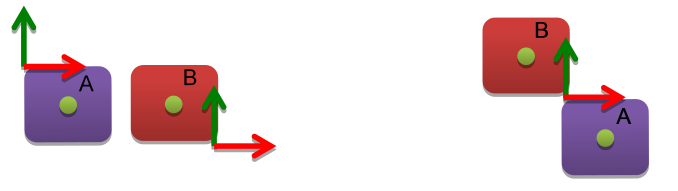
Fig. 12.1 Left, initial configuration. Right, relaxed configuration.¶

12.2. Ordinary constraints¶

Ordinary constraints (derived from the class agx::Constraint) are composites of elementary and secondary constraints. They can be used in a simulation to build up machines, such as cars, elevators etc. Ordinary constraints also consist of secondary constraints, which can define motors and limits. A body without constraints, is free to translate (t₁, t₂, t₃) and rotate (r₁, r₂, r₃), a total of 6 degrees of freedom (DOF). A constraint will restrict the motion of an attached body to one or more DOF.

For example, a Prismatic will allow a body to translate along one axis only, the other five DOF are constrained, while a LockJoint will restrict the movement of a body to all six DOF. Table 12.4 below show the number of degrees of freedom removed for each constraint.

Table 12.4 Degrees of freedoms removed for constraints¶
CONSTRAINT	#DEGRESS OF FREEDOMS REMOVED	#TRANSLATIONAL	#RATIONAL
Hinge	5	3	2
LockJoint	6	3	3
AngularJoint	3	0	3
Prismatic	5	2	3
CylindricalJoint	4	2	2
DistanceJoint	1	1	0
UniversalJoint	4	3	1
BallJoint	3	3	0
SplineJoint	4	2	2
WheelJoint	3	2	1

Table 12.5 lists each ordinary constraint with their respective elementary and secondary constraints.

Table 12.5 Elementary- and SecondaryConstraints usage for Constraints¶
Constraint	ElementaryConstraints	SecondaryConstraints
Hinge	1 x Spherical, 2 x Dot1	Range1D, Motor1D, Lock1D
LockJoint	1 x Spherical, 1 x QuatLock	None
AngularJoint	1 x QuatLock	None
Prismatic	1 x QuatLock, 2 x Dot2	Range1D, Motor1D, Lock1D
CylindricalJoint	2 x Dot1, 2 x Dot2	2xRange1D, 2xMotor1D, 2xLock1D
DistanceJoint	1 x Distance	Range1D, Motor1D, Lock1D
UniversalJoint	1 x Spherical, 1 x Dot1	Motor
BallJoint	1 x Spherical	None
SplineJoint	2 x Dot1, 2 x Dot2	2xRange1D, 2xMotor1D, 2xLock1D, 1xKinematic Body
WheelJoint	2x Dot2, 1x Dot1	4 x Range1D, 3 x Motor1D, 3 x Lock1D

Each constraint declares an enum, specifying an index for each DOF that it removes:

enum DOF
{
  ALL_DOF=-1,        /**< Select all degrees of freedom */
  TRANSLATIONAL_1=0, /**< Select DOF for the first translational axis */
  TRANSLATIONAL_2=1, /**< Select DOF for the second translational axis */
  TRANSLATIONAL_3=2, /**< Select DOF for the third translational axis */
  ROTATIONAL_1=3,    /**< Select DOF corresponding to the first rotational axis */
  ROTATIONAL_2=4,    /**< Select DOF corresponding to the second rotational axis */
  ROTATIONAL_3=5,    /**< Select DOF corresponding to the third rotational axis */
  NUM_DOF=6          /**< Number of DOF available for this constraint */
};

Which can be used as follows:

// Set the compliance for translational movements for the hinge:
hinge->setCompliance( 1E-8, Hinge::TRANSLATIONAL_1 );
hinge->setCompliance( 1E-8, Hinge::TRANSLATIONAL_2 );
hinge->setCompliance( 1E-8, Hinge::TRANSLATIONAL_3 );

Most constraints will also return the number of DOF it applies onto a body with the method:

// Get the number of DOF for this constraint. -1 if numDof is not defined for the constraint.
int numDof = hinge->getNumDOF();

12.3. Hinge¶

A Hinge removes 5 degrees of freedom from the constrained body allowing for rotation around an axis. A hinge has an angular range, lock and motor. The geometrical configuration of a hinge in AGX is defined by using Attachment frames (12.1.4). By default, a hinge revolves around the positive Z-axis.

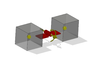
Fig. 12.2 Illustration of a hinge where (1) is the hinge center and (2) the axis. The bodies are free to rotate around this axis.¶

Hinge example 1: Create a single body hinge (connected to world)

// body1 is a rigid body
agx::FrameRef frame = new agx::Frame();
frame->setLocalTranslate( -1.0, 0.0, 0.0 ); // Hinge axis translated -1 along X

// Align hinge axis along negative y-axis instead of Z.
frame->setLocalRotate( agx::Quat(agx::Vec3::Z_AXIS(), agx::Vec3::Y_AXIS()*(-1)) );
agx::ref_ptr< agx::Hinge > h = new agx::Hinge( frame, body1 );

Hinge example 2: Connect two bodies with a hinge which reproduces the example from Fig. 12.2 assuming body1 is the one to the left:

// body1 and body2 are rigid bodies
agx::FrameRef frame1 = new agx::Frame;
agx::FrameRef frame2 = new agx::Frame;
frame1->setLocalTranslate( 1,0,0);
frame1->setLocalRotate( agx::EulerAngles(agx::degreesToRadians(90.0),0,0) );
frame2->setLocalTranslate( -1,0,0);
frame2->setLocalRotate( agx::EulerAngles(agx::degreesToRadians(-90.0),0,0) );

agx::HingeRef h = new agx::Hinge( body1, frame1, body2, frame2 );

Finally, to be realized, the constraint has to be added to the simulation.

simulation->add( h.get() );

12.4. Ball Joint¶

A ball joint removes the three translational degrees of freedom for a constrained body.

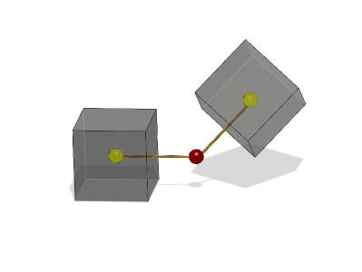
Fig. 12.3 Illustration of a Ball joint where the red sphere is the ball joint center.¶

Ball joint example 1: Create a single body Ball joint (connected to world) at the origo of the rigid body:

// body1 is a rigid body
agx::FrameRef frame = new agx::Frame();
agx::BallJointRef b = new agx::BallJoint(body1  frame);

Ball joint example 2: Connect two bodies with a Ball joint

// body1 and body2 are rigid bodies
agx::FrameRef frame1 = new agx::Frame();
agx::FrameRef frame2 = new agx::Frame();

frame1->setLocalTranslate(-1,0,0);
frame2->setLocalTranslate(1,0,0);

// Create A BallJoint using the two frames
agx::BallJointRef b = new agx::BallJoint( body1, frame1, body2,       frame2 );

simulation->add( b );

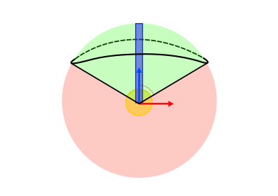
12.4.1. ConeLimit¶

A ball joint does not have a range limit, instead it has a cone limit. You can imagine it as if there is a cone in the frame of the base attachment, the z-axis of the other attachment is then limited to move inside that cone.

In the ball joint, the second attachment will always be the base attachment of the cone limit.

The cone limit has two limiting angles. Setting them to the same value will create a simple circular cone limit and setting them to different values will result in an elliptic cone limit. Note that the limit angles have to be smaller than \(\frac{\pi}{2}\).

// Enable cone limit, by default, limit angles are both PI/4
ballJoint->getConeLimit()->setEnable(true);

// Set limit angles
ballJoint->getConeLimit()->setLimitAngles(PI/4, PI/3);

12.4.2. TwistRangeController¶

The TwistRangeController limits how much an object can rotate around its own z-axis, relative to another object’s z-axis. Just as for the cone limit, the second attachment of the ball joint will always be seen as the base attachment, and the first one is what we limit relative to that one.

Note

The TwistRangeController fails when the z-axis of the frame is exactly opposite the z-axis of the reference frame. This controller is intended to be used together with the ConeLimit, where this cannot occur.

The range that can be set on the twist range controller is limited to be smaller than \(\pi\) and larger than \(-\pi\). Setting the angles to the same value will create a lock at that angle.

// Enable twist range, by default, it has no range set
ballJoint->getTwistRangeController()->setEnable(true);

// Set the range limit
ballJoint->getTwistRangeController()->setRange(-PI/4, PI/4);

12.4.3. FrictionControllers¶

The FrictionControllers in the ball joint works much in the same way as FrictionController - joint internal friction.The difference is that the ball joint contains multiple friction controllers. There is one for each of the three rotational degrees of freedom. The friction coefficient can be set individually on each of them, or it is possible to use the help functions on the ball joint to set it on all of them at once.

// Get the friction controllers of the different rotational directions
FrictionControllerRef frictionControllerU = ballJoint->getRotationalFrictionControllerU();
FrictionControllerRef frictionControllerV = ballJoint->getRotationalFrictionControllerV();
FrictionControllerRef frictionControllerN = ballJoint->getRotationalFrictionControllerN();

// Get all rotational friction controllers
FrictionControllerRefSetVector frictionControllers = ballJoint->getRotationalFrictionControllers();

// Enable and set friction coefficient to the same value on all rotational friction controllers
ballJoint->setEnableRotationalFriction(true);
ballJoint->setRotationalFrictionCoefficient(0.1);

There are two additional FrictionControllers that can be used to set friction on the cone limit. One controls the friction for sliding along the limit, and the other for rotating on the limit. These FrictionControllers can be accessed separately or all at once, just as with the rotational friction controllers.

// Get the specific friction controllers
FrictionControllerRef limitFrictionController = ballJoint->getConeLimitFrictionControllerLimit();
FrictionControllerRef rotationalFrictionController = ballJoint->getConeLimitFrictionControllerRotational();

// Get all the cone limit friction controllers
FrictionControllerRefSetVector frictionControllers = ballJoint->getConeLimitFrictionControllers();

// Enable and set friction coefficient to the same value on all cone limit friction controllers
ballJoint->setEnableConeLimitFriction(true);
ballJoint->setConeLimitFrictionCoefficients(0.1);

Note that if the cone limit is not active, the cone limit friction controllers will not apply any forces at all, since they are only active on the limit.

12.5. Universal joint¶

A universal joint transfer rotation via a central point through two rotation axes. The two rotation axes can be “bent” against each other. A universal joint is usually modeled with two hinges, however this requires an additional rigid body at the central point. The universal joint does not require this extra body. In addition the universal joint has motor, lock and range for the two remaining rotation dof’s.

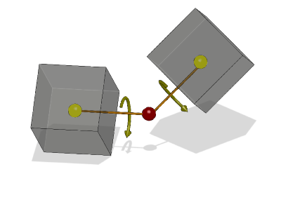
../_images/constraints_universaljoint.png

Fig. 12.5 Illustration of a Universal joint where the red sphere is the universal joint center and the orange sticks are the rotational axes for each body, (rotations about this axis is equal for both bodies). The bodies are free to move around the universal center and rotation about the universal axis is constrained (equal rotation).¶

Universal joint example: Connect two bodies with a Universal joint

// Creating a universal joint, axis along world z.
agx::FrameRef rbFrame = new agx::Frame();
rbFrame->setTranslate(0,0,1.5);
agx::FrameRef rb2Frame = new agx::Frame();
rb2Frame->setTranslate(0,0,-1.5);
agx::UniversalJointRef universal = new agx::UniversalJoint( body1, rbFrame, body2, rb2Frame );

Then to realize the constraint it has to add the constraint into the simulation:

simulation->add( universal );

12.5.1. Motor¶

A universal joint has two motors, one for each rotational axis which can be individually controlled:

// Enable the two motors
universal->getMotor1D( agx::UniversalJoint::ROTATIONAL_CONTROLLER_1 )->setEnable( true );
universal->getMotor1D( agx::UniversalJoint::ROTATIONAL_CONTROLLER_2 )->setEnable( true );

// Set a speed to the two motors
universal->getMotor1D( agx::UniversalJoint::ROTATIONAL_CONTROLLER_1 )->setSpeed( 0.5 );
universal->getMotor1D( agx::UniversalJoint::ROTATIONAL_CONTROLLER_2 )->setSpeed( 0.2 );

12.5.2. Range¶

A universal joint also has two ranges, one for each rotational axis:

// Enable the ranges
universal->getRange1D( agx::UniversalJoint::ROTATIONAL_CONTROLLER_1 )->setEnable( true );
universal->getRange1D( agx::UniversalJoint::ROTATIONAL_CONTROLLER_2 )->setEnable( true );

// Set the ranges
universal->getRange1D( agx::UniversalJoint::ROTATIONAL_CONTROLLER_1 )->setRange( -agx::PI*0.3, agx::PI*0.3 );
universal->getRange1D( agx::UniversalJoint::ROTATIONAL_CONTROLLER_2 )->setRange( -agx::PI*0.3, agx::PI*0.3 );

12.5.3. Lock¶

The universal joint also has a lock for each rotational axis:

// Enable the locks
universal->getLock1D( agx::UniversalJoint::ROTATIONAL_CONTROLLER_1 )->setEnable( true );
universal->getLock1D( agx::UniversalJoint::ROTATIONAL_CONTROLLER_2 )->setEnable( true );

// Set the lock positions
universal->getLock1D( agx::UniversalJoint::ROTATIONAL_CONTROLLER_1 )->setPosition(agx::PI);
universal->getLock1D( agx::UniversalJoint::ROTATIONAL_CONTROLLER_2 )->setPosition(agx::PI);

12.6. Prismatic universal joint¶

A prismatic universal joint is the same type of constraint as a universal joint but with an addition of a prismatic joint with its own motor, lock and range. Constructing a prismatic universal joint is analogue to all other joints.

// Creating a universal prismatic joint, axis along world z.
agx::FrameRef rbFrame = new agx::Frame();
rbFrame->setTranslate(0,0,1.5);
agx::FrameRef rb2Frame = new agx::Frame();
rb2Frame->setTranslate(0,0,-1.5);
agx::PrismaticUniversalJointRef universal = new agx::PrismaticUniversalJoint(
                                                                                                              body1, rbFrame, body2, rb2Frame );

Accessing the prismatic motor, range and lock is done through the same interface as for a universal joint:

// Enable the prismatic motor
universal->getMotor1D( agx::UniversalJoint::TRANSLATIONAL_CONTROLLER_1 )->setEnable( true );

// Set the force range and speed
universal->getMotor1D( agx::UniversalJoint::TRANSLATIONAL_CONTROLLER_1 )->setSpeed( 0.1 );
universal->getMotor1D( agx::UniversalJoint::TRANSLATIONAL_CONTROLLER_1 )->setForceRange(-100,100);

12.7. Distance joint¶

Distance joints remove one translational degree of freedom for a constraint rigid body. A Distance joint can also be seen as a spring. It will try to restore the distance between two attached rigid bodies. (Or an attachment point in the world and one rigid body). A Distance joint also has a motor which can push constrained bodies away or pull them together. This can be used to simulate a hydraulic actuator.

Distance joint example1: Connect one body to world with a Distance joint

// body1 is a rigid body
// Given in body frame
// Position in the world where the attachment of the distance joint is
agx::Vec3 worldConnectPoint( 0.0, 0.0, 10.0 );
agx::FrameRef frame = new agx::Frame(); // Other end of joint is at origo of rigid body
agx::DistanceJointRef d = new agx::DistanceJoint(body1, frame, worldConnectPoint);

Distance joint example 2: Connect two bodies to each other with a Distance joint and enable the motor:

// body1 and body2 are rigid bodies
agx::FrameRef frame1 = new agx::Frame()
frame1->setLocalTranslate(
agx::FrameRef frame2 = new agx::Frame()

agx::DistanceJointRef d = new agx::DistanceJoint(body1,frame1, body2, frame2);

// Disable the lock so that it will not interfere with the motor
d->getLock1D()->setEnable(false);

// Enable the motor and increase the distance between the two bodies with 0.1 m/s
d->getMotor1D()->setEnable(true);
d->getMotor1D()->setSpeed(0.1);

// set locked at zero speed, to avoid slipping when the distance is supposed to be constant
d->getMotor1D()->setLockedAtZeroSpeed(true);

12.8. LockJoint¶

A LockJoint will remove all six DOF from an attached body.

To lock a single body to the world or two bodies together it is possible to use the AGX Lock joint. Lock joint example 1: Connect one body to the world with a Lock joint

// body1 is a rigid body
agx::LockJointRef l = new agx::LockJoint( body1 );

simulation->add( l.get() );

Lock joint example 2: Connect two bodies to each other with a Lock joint

// body1 and body2 are rigid bodies
body1->setPosition( agx::Vec3( 10.0, 0.0, 0.0 ) );
body2->setPosition( agx::Vec3( 5.0, 0.0, 0.0 ) );
agx::Frame frame1 = new agx::Frame;
frame1->setLocalTranslate(-2.5,0,0);
frame2->setLocalTranslate(2.5,0,0);

agx::LockJointRef l = new agx::LockJoint(body1, frame1, body2, frame2);

simulation->add( l );

12.9. Prismatic¶

A prismatic constraint will remove 5 DOF from any attached rigid body. The body is free to translate along a specified axis. Compare to an elevator.

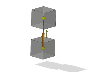
Fig. 12.6 Illustration of a Prismatic joint. Bodies are free to translate along one axis. No rotation is allowed around this axis.¶

12.10. CylindricalJoint¶

A CylindricalJoint is a 2D constraint. It consists of a hinge and a prismatic. It means that two degrees of freedom are left for a constrained body, one rotational and one translational. Basically, the constrained body can translate along the specified axis as well as rotating around it. Both has a motor, range and lock.

Special for the cylindrical constraint is that it also has a Screw1D secondary constraint (more about secondary order constraints in 12.15).

Each of the motors, locks and ranges can be accessed through the call:

agx::Motor1D* linearMotor = cylindrical->getMotor1D( agx::Constraint2DOF::FIRST );
agx::Motor1D* angularMotor = cylindrical->getMotor1D( agx::Constraint2DOF::SECOND );

12.10.1. Screw1D¶

The Screw1D secondary order constraint connects the prismatic (linear) and the hinge (rotational) part of a CylindricalJoint.

If you try to translate the constrained body, it will also start to rotate. The ratio between the translational movement and the rotational is specified through the call to setLead( agx::Real ):

// Create a Cylindrical joint (pseudo code)
agx::CylindricalJointRef cylindrical = new agx::CylindricalJoint(...);
// Enable the Screw1D
cylindrical->getScrew1D()->setEnable( true );

// For each revolution, the constrained body will translate 0.1 units.
cylindrical->setLead(0.1);

12.11. SplineJoint¶

A SplineJoint is a 2D constraint. It is related to the Cylindrical joint in that it consists of a hinge and a prismatic. In addition it also contains a hidden kinematic rigid body. This joint will limit translation along a specified spline. It means that two degrees of freedom are left for a constrained body, one rotational and one translational. Basically, the constrained body can translate along the specified spline as well as rotating around it. Both has a motor, range and lock which can be accessed in the same manner as the CylindricalJoint.

agxUtil::Spline* spline = new agxUtil::CubicSpline();
spline->add( agxUtil::Spline::Point(agx::Vec3(0,0,0)));
spline->add( agxUtil::Spline::Point(agx::Vec3(0,2,1)));
spline->add( agxUtil::Spline::Point(agx::Vec3(0,4,5)));
spline->updateTangents();

// Specifies a relative transformation between the spline point/tangent and the attached rigidbody
agx::FrameRef frame = new agx::Frame();

// Create the joint
agx::SplineJointRef joint = new agx::SplineJoint(body, frame, spline);

12.12. WheelJoint¶

A WheelJoint is a constraint to attach a wheel to a chassi or the world. The WheelJoint can be created in a few different ways. What they all have in common is that the wheel is the first body and the optional chassi is the second.

When using agx::Frames to construct a WheelJoint, some axes are more important than others. The Y-axis in the first body’s frame specifies the wheel axle. The Z-axis in the second body’s frame is used as suspension axis. When the steering is engaged, the rotation will be around this axis so it can also be referred to as steering axis.

The setup can also be done by using a WheelJointFrame which specifies in world coordinates, the wheel axis, the suspension/steering axis and the intersection point between those two. The two axes that are defined must be perpendicular.

agx::RigidBody* wheel = ... ;

// Position wheel at (1,0,0)
wheel->setPosition( agx::Vec3( 1.0, 0, 0 ) );

// We have the attachment between wheel axle and steering axle at (0.5, 0, 0)
agx::Vec3 worldAttach       = agx::Vec3( 0.5, 0, 0 );

// Wheel attachment point and wheel position are on the wheel axle
agx::Vec3 worldWheelAxle    = agx::Vec3( 1, 0, 0 );
agx::Vec3 worldSteeringAxle = agx::Vec3( 0, 0, 1 );

// Specify a frame
auto wheelJointFrame = WheelJointFrame( worldAttach, worldWheelAxle, worldSteeringAxle );

// Create the constraint. In this case, the wheel is attached to the world
agx::WheelJoint* wheeljoint = new agx::WheelJoint( wheelJointFrame, wheel, nullptr );

simulation->add( wheeljoint );

// The suspension is locked by default, release...
auto su_lock = wheeljoint->getLock1D( agx::WheelJoint::SUSPENSION );
su_lock->setEnable( false );

// .. and enable the range instead to show free movement.
auto su_range = wheeljoint->getRange1D( agx::WheelJoint::SUSPENSION );
su_range->setEnable( true );
su_range->setRange( -0.1, 0.1 );

// If we don't want rotation around the steering axis, we can lock it
// at its current angle
auto st_lock = wheeljoint->getLock1D( agx::WheelJoint::STEERING );
st_lock->setPosition( wheeljoint->getAngle( agx::WheelJoint::STEERING) );
st_lock->setEnable( true );

12.12.1. Connecting to a power-line¶

A WheelJoint can be powered by a power-line by attaching it to an Actuator. A RotationalActuator cannot be used by itself since a WheelJoint has multiple degrees of freedom, which means that we need to tell the Actuator which of them it should operate on. This is done by passing a WheelJointConstraintGeometry to the RotationalActuator. The WheelJointConstraintGeometry identifies one of the WheelJoint’s free degree of freedom and we chose which one using the same technique as when getting a Lock1D or a Range1D from it.

Continuing the example above.

agxPowerLine::ConstraintGeometryRef wheelAttachAxis =
  new agxVehicle::WheelJointConstraintGeometry(wheelJoint, agxVehicle::WheelJoint::WHEEL);
agxPowerLine::RotationalActuatorRef actuator =
  new agxPowerLine::RotationalActuator(wheelJoint, wheelAttachAxis);

To control the suspension with a TranslationalActuator we would use agxVehicle::WheelJoint::SUSPENSION instead.

agxPowerLine::ConstraintGeometryRef suspensionAttachAxis =
  new agxVehicle::WheelJointConstraintGeometry(wheelJoint, agxVehicle::WheelJoint::SUSPENSION);
agxPowerLine::RotationalActuatorRef actuator =
  new agxPowerLine::RotationalActuator(wheelJoint, suspensionAttachAxis);

For more information on power-line components and how to connect them see AGX PowerLine. For a complete example see the tutorial_wheel_joint.agxPy Python tutorial.

12.13. Steering¶

When a car actually turns as shown in Fig. 12.7 a), the steering mechanism is designed to align the wheels simultaneously. The inner wheel will follow a circle with radius \(R\), while the outer wheel follows a concentric circle with radius \(R + W_t\). Note that \(W_t\) refers to the wheel track, \(W_b\) denotes the wheel base.

To minimize the slip and ensure the better turning performance, the front steerable wheels should hold the different steering angles of \(\delta_{\text{in}}\) and \(\delta_{\text{out}}\). According to Ackermann principle, it yields

\[\delta_{out} = \arctan\left(\frac{1}{\cot(\delta_{in}) + W_t/W_b}\right)\]

where \(\delta_{\text{in}}\) refers to the steering angle of the inner wheel, \(\delta_{\text{out}}\) is the ideal steering angle of the outer wheel corresponding to the prescribed \(\delta_{\text{in}}\).

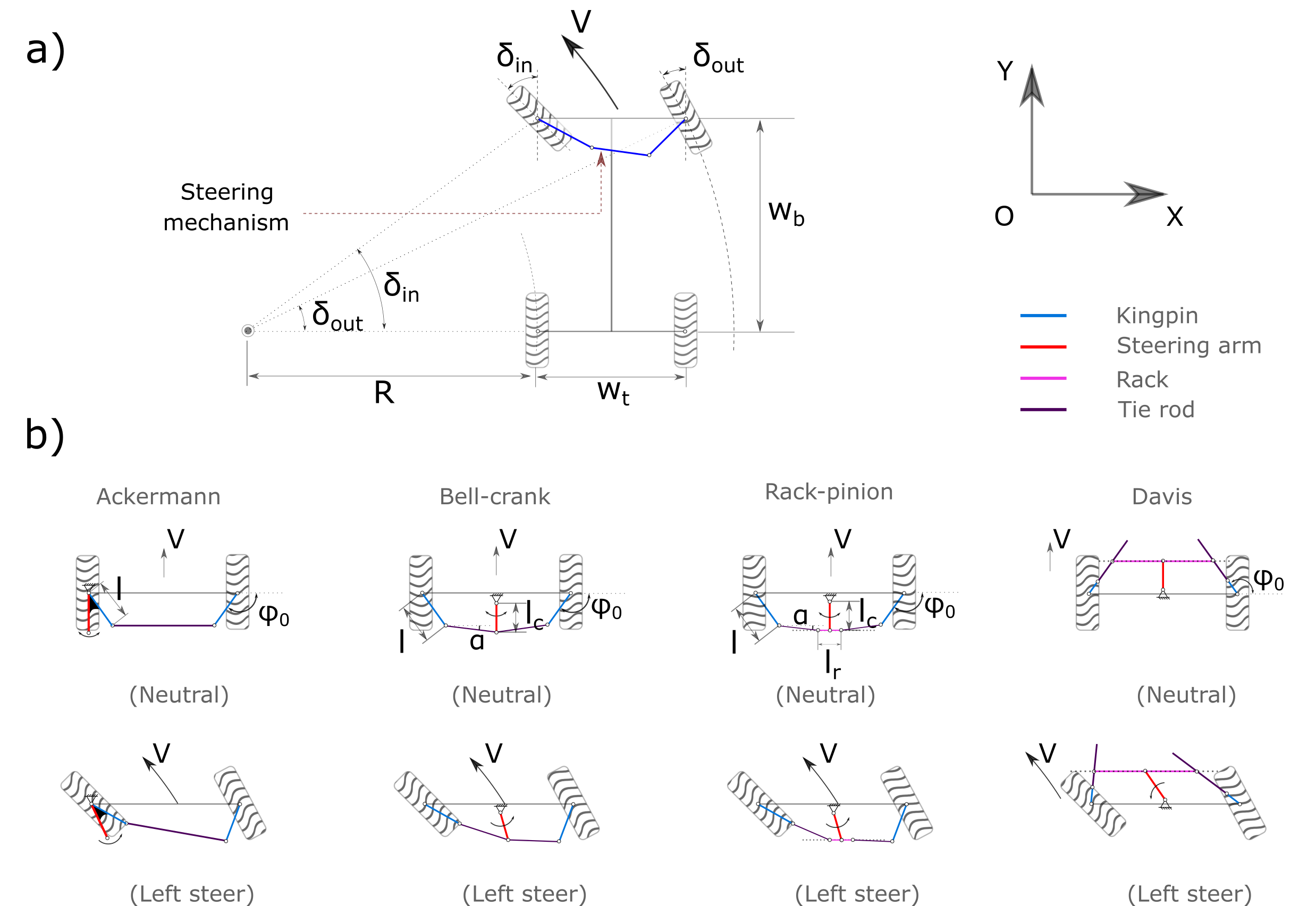
Fig. 12.7 Car steering schematic. a) Turning geometry; b) Four different steering mechanisms.¶

The generally used Ackermman steering mechanism (See Fig. 12.7 b)) is a symmetric planar four-bar linkage. The steering arm, which rigidly connects but not limited to the left kingpin, will transmit the direct steering input of steering wheel to the two front steerable wheels via the trapezoid four-bar linkage. The Ackermann steering geometry is known to be simple and easy for calculation. But it is not always practically possible to implement. Alternatively, there are other steering mechanisms such as bell-crank (also called central-lever [7]), rack-pinion, and davis proposed.

For instance, in a bell-crank steering system, the steering arm rotates, pushing the shared ends of the tie rods to move left or right. This in turn will cause the wheel to turn due to the steering linkages. Bell-crank steering has been reported [7] that is common to wheeled tractors, ATVs, etc.

Regarding the Rack-pinion steering mechanism, the pinion is used to transmit the angular motion of the steering arm into the translational or linear motion of the rack. Rack-pinion steering mechanism is most commonly used to passenger cars [9].

Davis steering mechanism [10] is an exact steering mechanism but is seldom used in practice. It has two sliding pairs in-between the tie rod and the bar. The tie rods are only allowed to move in the direction of the its length. The main disadvantage of the Davis steering is the wear problem of the sliding pairs.

There four abovementioned steering mechanism have all been implemented and are now available in AGX Dynamics.

12.13.1. Geometrical parameters¶

As can be seen from Fig. 12.7 b), all the steering mechanisms share the common parameters of \(\phi_{0}\) and \(gear\). The meaning of these parameters have been described in Table 12.6 as shown below. It can be noticed that the number of independent geometrical parameters varies in terms of the steering mechanisms. For example, there are only one independent parameter of \(\phi_{0}\) needed for Davis steering, and two parameters of \(\phi_{0}\) and \(l\) for Ackermann steering to define the steering geometry. The steering parameters as listed in Table 12.6 are default and optimal. They were selected from [7], [8], [11] and [12].

Table 12.6 Default steering parameters in AGX Dynamics¶
Parameter	Unit	Description	Ackermann	BellCrank	RackPinion	Davis
\(\phi_{0}\)	rad	Angle between kingpin direction and X axis	\(\frac{-115}{180}\pi\)	\(\frac{-108}{180}\pi\)	\(\frac{-108}{180}\pi\)	\(\frac{104}{180}\pi\)
\(l\)	\(\frac{1}{W_t}\)	kingpin length	0.16	0.14	0.14	–
\(\alpha\)	rad	Angle between tie rod and X axis	–	0.0	0.0	–
\(l_c\)	\(\frac{1}{W_t}\)	Steering arm length	–	1.0	1.0	–
\(l_r\)	\(\frac{1}{W_t}\)	Rack or bar length	–	–	0.25	–
gear	–	Steering wheel gear ratio	1.0	1.0	1.0	1.0
side	–	Side of steering arm positioned	0	–	–	–

In Table 12.6, "-" indicates that is not applicable.

The users can build their own desired steering geometry using the customized steering geometry parameters. For instance,

auto steerParams = new agxVehicle::SteeringParameters();
// The different values of parameters from the default are prescribed.
steerParams->phi0 = agx::degreesToRadians(-115);
steerParams->l = 0.16;

auto ackermann = new agxVehicle::Ackermann( leftWheel, rightWheel, steerParams);
sim->add( ackermann );

Once the steering mechanism is active, the range of the maximum allowed turning angle according to the geometrical configuration of the steering mechanism will be enabled automatically. This range should not be modified or disabled by the user. Howeever, the user can access the maximum allowed steering angle using the getMaximumSteeringAngle() method.

12.13.2. Building steering¶

All the steering mechanisms implemented are enforced as three body constraints between each wheel body and the chassi.

The steering mecanisms can be created by simply replacing the “BellCrank” as shown below with the others such as “RackPinion”, “Davis” and “Ackermann”.

SteeringRef steeringMechanism = new agxVehicle::BellCrank( leftFrontWheel, rightFrontWheel );
sim->add( steeringMechanism );

If no SteeringParameters are assigned as an input after the “rightWheel”, the default steering parameters as listed in Table 12.6 will be used.

12.13.3. Steering manipulation¶

The steering can be manipulated using the setSteeringAngle() method.

class steeringListener : public agxSDK::StepEventListener
{
  public:
    steeringListener(agxVehicle::Ackerman* ackermann) :
    {
    }
    void pre(const agx::TimeStamp& t)
    {
      if (t < 1.0) {
        ackermann->setSteeringAngle(t);
      }
      else if (t <= 3.0) {
        ackermann->setSteeringAngle(1 - (t-1) / 2);
      }
      else
      {
        ackermann->setSteeringAngle(0.0);
      }
    }

Detailed C++ and python examples with the abovementioned steering mechanisms are available in tutorials/agxVehicle/tutorial_carSteering.cpp and python/tutorials/tutorial_carSteering.agxPy.

12.14. Constraint Forces¶

It is possible to read forces applied by a constraint. For more details, see 11.20.2.

12.15. Secondary order constraints¶

Secondary constraints are constraints on constraints such as limits and motors. The Secondary constraint will operate on the DOF which is not constrained. For example, a Hinge allows a body to rotate around one axis. The Secondary constraints of a Hinge will operate on that DOF.

Different constraints have different secondary order constraints. For example, a Hinge has Lock1D, Motor1D and Range1D secondary constraint while LockJoint does not have any secondary constraint at all. The secondary constraints can be requested through a call to the constraint API:

agx::Motor1D* motor = hinge->getMotor1D();
agx::Lock1D* lock = hinge->getLock1D();
agx::Range1D* range = hinge->getRange1D();

The CylindricalJoint (12.10) has one additional secondary constraint:

agx::Screw1D* screw1D = cylindrical->getScrew1D();

12.15.1. Motor1D¶

Motor1D is a controller which operates on the free degree of freedom for a constraint such as the rotational axis of a Hinge, the sliding axis of a Prismatic and or the rotational/sliding axis of a CylindricalJoint. A motor can be speed controlled either by specifying a speed or a force/torque, or both:

hinge->getMotor1D()->setSpeed( 1.2 ); // Set the desired speed in radians/sec
// Specify the available amount of torque in negative and positive direction
hinge->getMotor1D()->setForceRange( -1000, 1000 );  // Nm

A motor for a rotational constraint such as a hinge has the units of rotational speed and torque, whereas a linear constraint such as a prismatic uses linear distance and force.

A motor is a velocity constraint; it will apply a force/torque to reach the desired speed. This means that a Motor1D will not be able to keep a constrained system stationary over time. It will be subject to a drift in position. To keep a constraint at a specified position, the Lock1D secondary constraint should be used.

The Motor1D however has a utility method called setLockedAtZeroSpeed() which will automatically transform the Motor1D to a Lock1D when the desired speed is zero:

// Whenever the desired speed is set to 0, the motor1d will operate as a Lock1D
// The same force range will be used for locking the constrained bodies.
hinge->getMotor1D()-setLockedAtZeroSpeed( true );

12.15.2. Lock1D¶

Lock1D can be used to lock a constrained body to a specific position. A specified force/torque range can be given which will limit the max force/torque that the lock can apply to maintain the desired position.

A Lock1D can for example be used to specify a wounded spring:

// Specify a position of -100 radians, ie. a wounded up spring.
hinge->getLock1D()->setPosition( -100 );
hinge->getLock1D()->setCompliance( 1E-5 );

12.15.3. Range1D¶

Range1D defines a valid range for a constrained rigid body to move around/along the specified axis. At the limits of a range you effectively get a contact behavior. By default the limits are –inifinity, +infinity.

// Enable the range
hinge->getRange1D()->setEnable( true );
// Specify the range limits
hinge->getRange1D()->setRange( agx::RangeReal(-agx::PI, 10*agx::PI) );

The above code would limit the rotation of a body between PI and 10 PI radians.

12.15.4. FrictionController - joint internal friction¶

The FrictionController is valid and available for Hinge (rotational), Prismatic (translational) and CylindricalJoint (rotational and translational), and adds an internal friction force such that:

\[F_{friction} \leq \mu F_{normal}\]

Note that for Hinge and rotational CylindricalJoint we’ve a resulting torque. For the friction condition to be dimensionally correct, the axle radius should be included in the friction coefficient, giving:

\[\tau_{friction} \leq \mu r F_{normal}\]

We have stick friction mode when \(F_{friction} < \mu F_{normal}\) and the objects are sliding when \(F_{friction} = \mu F_{normal}\).

The friction controller is disabled by default.

// Enable the friction controller in the hinge.
hinge->getFrictionController()->setEnable( true );
// Assign friction coefficient: Default: 0.4167
hinge->getFrictionController()->setFrictionCoefficient( 0.25 );

// Enable friction controller and set friction coefficient in the cylindrical translational part.
cylindrical->getFrictionController( agx::Constraint2DOF::FIRST )->setEnable( true );
cylindrical->getFrictionController( agx::Constraint2DOF::FIRST )->setFrictionCoefficient( 0.7 );

// Enable friction controller and set friction coefficient in the cylindrical rotational part,
// including axle radius.
agx::Real axleRadius = 0.025;
cylindrical->getFrictionController( agx::Constraint2DOF::SECOND )->setEnable( true );
cylindrical->getFrictionController( agx::Constraint2DOF::SECOND )->setFrictionCoefficient( 0.15 * axleRadius );

12.15.4.1. Minimum static friction¶

The friction controller includes a setting for minimal static friction force, meaning there is a friction restistance even with the friction coefficient set to zero.

// Enable the friction controller in the hinge.
hinge->getFrictionController()->setEnable( true );
// Assign minimum static friction torque to 10Nm for both rotational directions: Default: agx.RangeReal(0,0).
hinge->getFrictionController()->setMinimumStaticFrictionForceRange( agx.RangeReal(-10,10 );

If you also specify a friction coefficient the friction force may exceed the static friction limit, \(F_{friction} = max(\mu F_{normal}, F_{minimum static friction})\).

12.15.4.2. Normal force¶

The normal force is calculated differently depending on which type of constraint the friction controller is active in. Given the constraint axis is defined to be along/about z, the normal force is defined to be translational constraint force along x (\(F_{normal}^x\)) and y (\(F_{normal}^y\)), which gives us the normal force:

\[F_{normal} = \sqrt{(F_{normal}^x)^2 + (F_{normal}^y)^2}\]

12.15.4.3. Linear and non-linear modes¶

The friction force depends on the normal force and in some non-trivial scenarios the normal force depends on the friction force. A simple and performance wise fast approach is to use the normal force from the previous time step to calculate the maximum friction force in the current time step. This is the default mode and will not significantly affect the performance but may affect the accuracy of the simulation. E.g., the first time step the friction forces will be zero since there’s no information regarding previous normal force.

For constraint solve types agx::Constraint::DIRECT and agx::Constraint::DIRECT_AND_ITERATIVE the friction controller supports non-linear update of the friction forces given current normal force. This mode is similar to direct friction for contacts and will affect the performance but will also increase the accuracy of the simulation. To enable non-linear mode:

// By default: constraint->getFrictionController()->getEnableNonLinearDirectSolveUpdate() == false
constraint->getFrictionController()->setEnableNonLinearDirectSolveUpdate( true );

12.15.5. Current Position¶

The secondary constraints has a current angle/position which can be queried with the call to getAngle(). For a hinge the call is:

// Get the current angle in radians
agx::Real currentAngle = constraint->getAngle();

And for a prismatic constraint:

// Create a prismatic
agx::Constraint1DOFRef constraint = new agx::Prismatic(...);

// Same call but here we get the current position as it is a Prismatic constraint
agx::Real currentPosition = prismatic->getAngle();

Notice that for a hinge, the angle is aware of winding. This means that the whole API for accessing/setting angles can accept values larger than 2*PI.

12.15.6. Current force¶

The current force applied by a secondary constraint can be accessed by a call to getCurrentForce, notice that the method is the same for both linear and angular constraints.

// Get the current torque applied by the hinge
agx::Real currentTorque = hinge->getMotor1D()->getCurrentForce();

For more details, see 11.20.2.

12.15.7. Regularization parameters for secondar constraints¶

The regularization parameters can be used to model the effect of a Secondary constraint. For example, when a hinge constraint reaches a limit, what parameters are then used? Should it be a stiff limit? (Compliance reaches zero) or a softer limit (compliance> 0). Should the limit be fulfilled immediately, (damping=0), or will we allow violation for some time (damping > 0).

// Specify how stiff the limit should be:
hinge->getRange1D()->getRegularizationParameters()->setCompliance(1E-5);

// Specify the damping of the limit
hinge->getRange1D()->getRegularizationParameters()->setDamping(3.0/60);

12.16. Rebind¶

The geometry configuration of a constraint can be changed during runtime, the attachment frames can be modified, bodies can be moved relative to each other, however this requires a call to Constraint::rebind() which will use the new configuration as the initial configuration. The result is a relaxed system where the bodies are at their current/modified transformation.

Observe that explicitly transforming dynamic objects during a simulation can have unwanted results: instability, missing collision detection, large constraint violations etc.

12.17. Solve type¶

The solver allows a great flexibility when it comes to configuring constraints. A Constraint can be set to be solved in the iterative/direct/both solvers with the method:

Constraint::setSolveType( Constraint::SolveType solveType );

Solving a constraint in the iterative solver, means that it will have a lower maximum compliance, i.e. it will be softer/more springy. The direct solver is able to handle very stiff constraints. The benefit of solving constraints in the iterative solver, is commonly it is faster. So depending on your specific configuration of your system, some constraints can be iterative and some can be direct.

It is however important that constraints that connects two subsystem where one is solved with the iterative and the other with the direct solver is set to DIRECT_AND_ITERATIVE. This is necessary to transfer the correct forces between the two subsystems. If not, the system can become unstable.

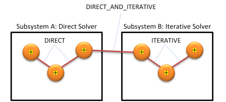
Fig. 12.8 Coupling between subsystems. (Red lines indicate constraints between bodies)¶

12.18. Constraint utility methods¶

The class Constraint also has a number of utility methods for creating constraint configurations:

Given two rigid bodies, a point in the world and an axis, the method below will compute the two attachment frames to create a relaxed system:

agx::Vec3 worldPoint(0,0,0); // Anchor point for the constraint
agx::Vec3 worldAxis(agx::Vec3::Y_AXIS()); // Axis for the constraint

agx::Constraint::calculateFramesFromWorld(worldPoint, worldAxis, body1, frame1, body2, frame2 );

// Create a hinge with the rotation axis along Y
agx::HingeRef hinge = new agx::Hinge(body1, frame1, body2, frame2);

12.19. Virtual Inertia¶

12.19.1. Basic usage¶

Virtual inertia and mass can be added to constraints along or about the central constraint axis (N-axis) to add resistance to acceleration on the bodies in the constraints. The dynamics in the constraint axis will then behave as though it has to move an extra mass and/or inertia. This can be used to emulate mechanisms, that are modeled using a single constraint, that have internal inertia.

Both translational mass and rotational inertia can be added separately, affecting the translation and rotational acceleration in the axis accordingly. However, the extra inertia/mass must act through one or more of the RigidBodies active in the constraint. This means that the user must decide how it should be distributed, which can be done in the constructor.

The virtual inertia is applied through an external class. The constructor takes the following arguments:

Argument	Description
constraint	The constraint that the virtual inertia should be active on.
rigidBody1TranslationInertia	The virtual mass in kg that will act on RigidBody 1 along the constraint translational axis.
rigidBody1RotationalInertia	The virtual inertia in kg*m2 that will act on RigidBody 1 about the rotational direction in the constraint axis.
rigidBody2TranslationInertia	The virtual mass in kg that will act on RigidBody 2 along the constraint translational axis.
rigidBody2RotationalInertia	The virtual inertia in kg*m2 that will act on RigidBody 2 about the rotational direction in the constraint axis.

12.19.2. Virtual Inertia in C++¶

The following code snippet demonstrates how to add virtual inertia to a hinge constraint with two active bodies. This will cause angular acceleration about the central hinge axis to be affected by an extra total inertia of 1 kg*m2. The inertia is added on the second body in the constraint, which means that only that body will feel the extra inertia. The virtual inertia can also be distributed evenly on the bodies, where both will be affected by half of the total inertia.

// Create a hinge constraint between two rigid bodies
agx::Frame* frame1 = new agx::Frame(); // empty frame
agx::Frame* frame2 = new agx::Frame(); // empty frame
agx::RigidBody* body1 = new agx::RigidBody(new agxCollide::Geometry(new agxCollide::Box(agx::Vec3(1.0,1.0,1.0))));
agx::RigidBody* body2 = new agx::RigidBody(new agxCollide::Geometry(new agxCollide::Box(agx::Vec3(1.0,1.0,1.0)))) ;
agx::Hinge* hinge = new agx::Hinge(body1, frame1, body2, frame2 );

/**
Add virtual inertia to the constraint to create artificial resistance to acceleration in the constraint axis.
Virtual inertia can be added in the translational and rotational general constraint axis direction.

The translational virtual inertia will resist acceleration along the constraint N-axis direction (extra mass) and the
rotational virtual inertia will resist rotational acceleration around the constraint N-axis direction.

This example adds rotational inertia to the hinge constraint adding a "virtual resistance" to rotational acceleration
in the hinge axis.
**/
agx::VirtualConstraintInertia* virtualInertia = new agx::VirtualConstraintInertia(hinge, 0, 0, 0, 1.0);

simulation->add( virtualInertia );

The following code snippet demonstrates how to add virtual inertia to a prismatic constraint with two active bodies. This will cause a resistance to acceleration along the prismatic axis. The extra mass is added evenly to both bodies.

// Create a prismatic constraint between two rigid bodies
agx::Frame* frame1 = new agx::Frame(); //empty frame
agx::Frame* frame2 = new agx::Frame(); //empty frame
agx::RigidBody* body1 = new agx::RigidBody(new agxCollide::Geometry(new agxCollide::Box(agx::Vec3(1.0,1.0,1.0))));
agx::RigidBody* body2 = new agx::RigidBody(new agxCollide::Geometry(new agxCollide::Box(agx::Vec3(1.0,1.0,1.0))));
agx::Prismatic* prismatic = new agx::Prismatic(body1, frame1, body2, frame2 );

/**
Add virtual inertia on both bodies in the translational direction (N-axis) of the constraint.
**/
agx::VirtualConstraintInertia* virtualInertia = new agx::VirtualConstraintInertia(prismatic, 0.5, 0, 0.5, 0);

simulation->add( virtualInertia );