
Reliable nonsmooth multidomain dynamics simulation
Numerical physics
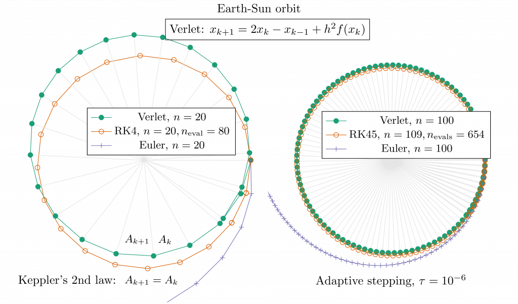
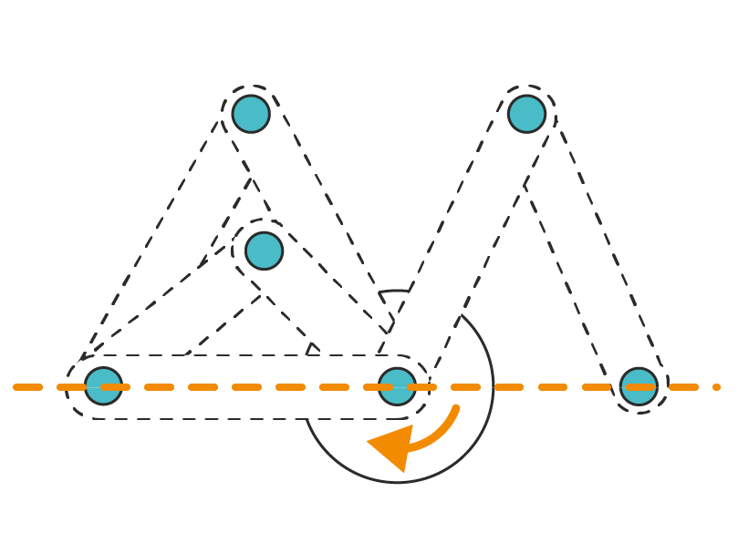
The discrete time variational principle of mechanics leads to numerical methods which preserve symmetries and are stable at large fixed steps. Applied to multibody and nonsmooth systems these new methods outperform general purpose ones by orders of magnitude.
Their numerical errors are unbiased and predictable globally and the trajectories are bounded for arbitrarily large time intervals.
And the time step can be safely set in direct proportion with the time scales of interest.
Fast, stable, robust
The stepper is implicit with a time symmetric linearization and is provably stable. This means the simulation time is predictable as needed for realtime applications.
The solver never breaks down due to degeneracy because of physical regularization which is a small compliance. The factorizer is an order of magnitude faster than the commonly used ones, and hybrid methods provide scalability.
The solver does not fail, by design.
Nonsmooth, multidomain
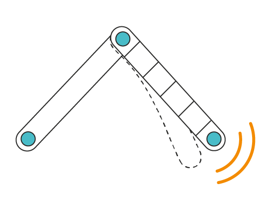
Impacts, contacts, dry friction are best modeled with hard inequalities solved implicitly. This is nonsmooth mechanics, the foundation of AGX.
With discrete time analytical mechanics, all physical domains are modeled uniformly, coupled via boundary conditions.
The two together leads to strong and stable coupling between all modules, from multibody to wires, via hydraulics and more.
AGX is much more than multibody.
AGX Dynamics: numerical simulation of nonsmooth multibody and multidomain dynamics.
Real physics for digital worlds
AGX Dynamics computes the the equations of motion of 3D multibody systems dynamics subject to impacts, contacts and friction, along with tightly coupled components from other physical domains such as hydraulics, drivelines, wires, etc. It is deeply integrated with a geometric computation kernel which automatically detects contacts between bodies according to 3D shapes they are connected to. It is true to life because it can handle non-ideal models of joints with gaps and elasticity for instance.
The science and the math
It works with a fixed time step so the computation times are predictable. That makes it suitable for real time applications, from interactive virtual environments to hardware in the loop cases. It is very stable so the time step can be large, and be adjusted according to time scales of interest without worries.
Use cases
Use cases range from simulator training, to testing and developing control systems, to prototyping and analysis of mechanical designs, and in Machine Learning (ML) applications for developing autonomous drivers for instance
It is designed to simulate over indefinitely long times. For instance, a continuous run over 40 hours for a training session is not only just fine but a typical usage. It is also dynamic: bodies can be added and deleted during a simulation, arbitrarily many contacts can be generated, and user interaction is expected. Users can even change the scene during an integration step at a number of stages during the computation pipeline. With full journaling capability, offline simulations can be played back in real-time.


AGX Dynamics computes the the equations of motion of 3D multibody systems dynamics subject to impacts, contacts and friction, along with tightly coupled components from other physical domains such as hydraulics, drivelines, wires, etc. It is deeply integrated with a geometric computation kernel which automatically detects contacts between bodies according to 3D shapes they are connected to. It is true to life because it can handle non-ideal models of joints with gaps and elasticity for instance.
Direct solver
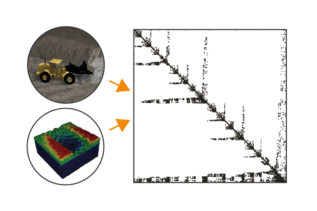
A direct solver based on a high performance sparse factorizer and a direct pivoting methods to handle inequalities delivers hard contacts and true stiction, allowing stable grasping. It provides stability under large mass ratios as well as high accuracy. A hybrid solver combines this with iterative methods in a flexible, configurable way, and delivers scalable performance for very large systems such as for nonsmooth DEM (NDEM) based granular matter. The user gets to choose which variables are processed by the direct solver, the iterative one, or both. This way, a 10 tonnes wheel loader can easily drive over a pile of granules of a few grams each without problems.
Solver
To protect the solver against degeneracy and keep condition numbers reasonable, an arbitrarily small compliance is built into the fundamental physical model and discretized in time with the variational principle. It therefore has a physical meaning and can be used to model linear elasticity for any function defined from the kinematics. Unlike penalty models coupled with standard implicit integrators, small compliance or high stiffness does not introduce anomalies in the physics such as excessive damping, or a large discrepancy between the simulated dynamics and the analytical model. The necessary damping is optimal by default and needs no tuning. The factorizer does not need to introduce further regularization during factorization, and does not even need to pivot because of novel technique for fill reducing reordering, leading to performance close to the maximum theoretical limit.
Models
Impacts, contacts and stiction are common in daily life and useful in designs. These are all discontinuous or nonsmooth for short. Commonly used mathematical models of multibody systems dynamics rely on continuity assumption, so do most commonly used numerical methods, and this is often problematic for performance. Not AGX Dynamics, however, as it is designed to handle real life scenarios, not idealized abstractions.
Based on analytical systems dynamics for modeling and the nonsmooth discrete time variational principle for stepping, it has multidomain capabilities and stable time integration with second order accuracy. Rigid bodies, hydraulic pipes and valves, electric motors, wires and cables are all the same thing in this framework, leading to unified, tightly coupled simulations. This combination of models and numerical methods is based on the most recent scientific literature from theory and modeling to numerical methods, to computer science.
Nonsmooth modeling allows for gaps or clearance in joints, granular matter with Discrete Element Models (DEM)s, elasto-plastic beams, joint limits, breakable joints, pressure compensated hydraulic pumps, piecewise linear models and much more. This is what real-life is made of. Why simulate idealized models?
The nonsmooth stepper does not slow down during an impact, when yield criteria are reached, or when a valve shuts. It resolves these conditions implicitly so that all inequalities are satisfied globally and consistently at each step. This combination of nonsmooth models from analytic system dynamics and nonsmooth stepper can regularly deliver three orders of magnitude in speedup as compared to standard ones using smooth formulations, adaptive stepping, and force-velocity coupling instead of hard constraints and algebraic conditions as done in AGX.
Time stepper
The time stepping method is implicit and is stable over indefinitely long simulation time. It is second order accurate, and can take larger steps than standard techniques. As we mostly consider non-smooth systems with discontinuities, higher order methods are neither required nor suitable. Multistep methods for instance would require at least the same amount of work per step and deliver higher accuracy. But they are entirely ill suited as they need to restart at each discontinuity. The step-size in AGX can be safely put to a value that is commensurate with the time and length scales of the dynamics of interest, leading to good accuracy. That is usually as large as the most popular Runge-Kutta methods which are much more expensive numerically for equivalent stability and step-size, up to six time slower when adaptive step size is considered. For similar accuracy, the AGX stepper often works no harder than higher order methods. And as said, high order methods on discontinuous equations is not a good idea.
To solve the implicit equations we linearize symmetrically in time which helps preserve energy and keep error unbiased. To compensate for the linearization a small amount of numerical damping time constant is required. This serves to filter high frequencies of stiff forces and stabilize constraints. This parameter has a known optimal value and requires no tuning. The energy lost due to this is predictable.
As we use augmented coordinates, systems with closed kinematic loops are not an issue, and constraint singularities are resolved via compliance.
Joints
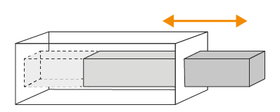
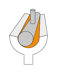
A library of joints and constraints is provided and should be sufficient for most applications. Nonholonomic constraints can be used to model simple motors, drivers and joint friction. All constraints can be relaxed to introduce linear elasticity, range limits can be put the motion itself, or on the forces which maintain joints and constraints so they can break when a given maximal load is reached. It is possible to extend this library using elementary components. Any function of the kinematic states of two or more bodies can be used to define a constraint or a potentially stiff force which is then integrated implicitly. Also in the library are slack joints, as needed for true to life applications.
Users can define their own functions from the kinematic relationships between two or more bodies. Jacobians are automatically computed if one uses the provided library of elementary functions. This way, one can implement new joints or stiff forces, with minimal headaches.
Geometry, collision detection and contact generation
Meshes
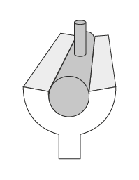
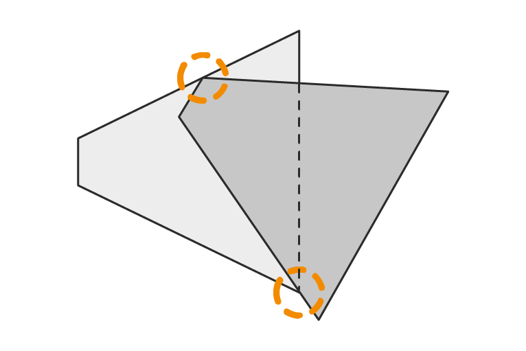
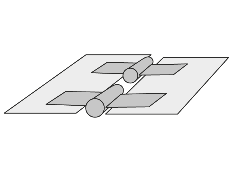
AGX was designed for interactive 3D applications and therefore contains geometry kernels to detect interferences and compute overlaps between objects and generate sets of contact points for the solver to process. Unstructured meshes are a fact of life but lead to expensive computations. Therefore, geometries can also be represented with primitives such as boxes, spheres, capsules and cylinders, or as convex meshes, height fields. And of course, composites made of these. Recent developments even include peg-in-hole type of contacts for conic shapes.
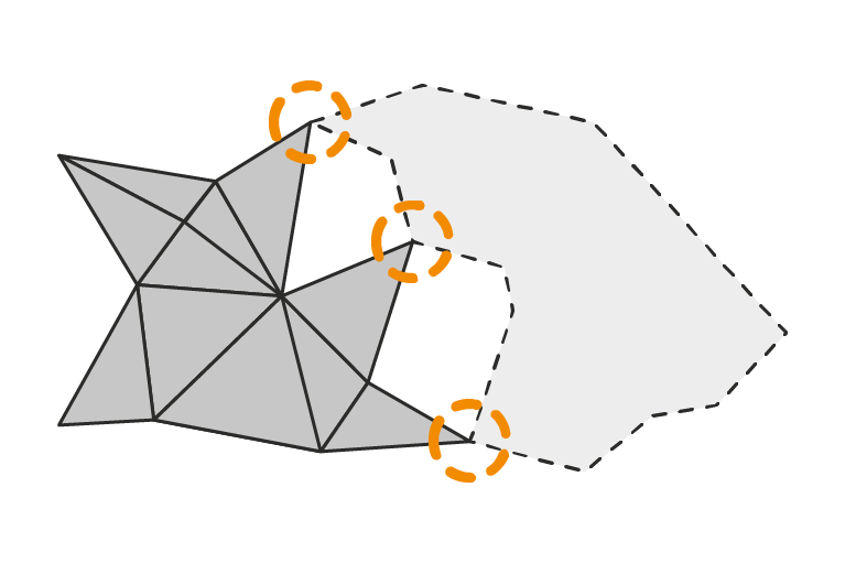
Meshes can cause serious performance problems but AGX contains a novel method to filter contacts and discard as many redundant ones as possible. AGX uses mostly point-wise contacts but there is some functionality to define surface models which account for Young’s and Bulk modulus.
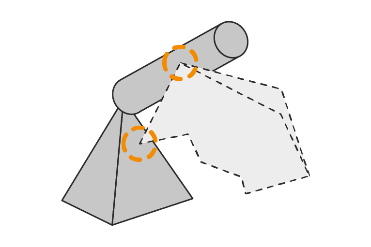
In addition to providing the standard array of algorithms from computational geometry as well as detection and contact generation kernels for all pairs of primitives, the library includes an algorithm which culls redundant contact points which greatly improves performance. In addition, peg-in-hole functionality has recently been added to the repertoire, which is a significant distinguishing factor.
AGX uses both point-wise and surface contact models making it possible to account for Young’s and Bulk moduli.
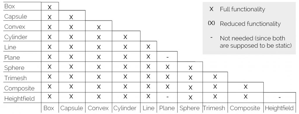
Collider types
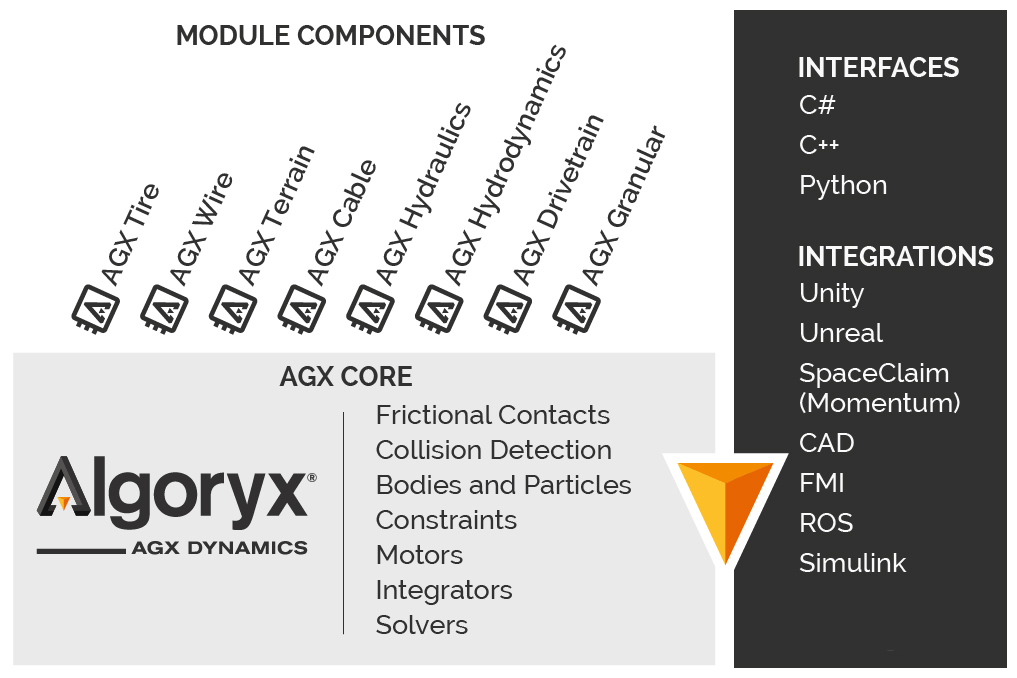
AGX Co-Simulation & Interface Integration with Software and Hardware Platform
AGX Dynamics has been successfully integrated with many industry leading software and hardware platforms such as Simulink and Robotstudio. Users can also access AGX Dynamics through various scripting languages, including C#, Lua and Python, and through the 3D modeling and authoring environments SpaceClaim and Unity. Co-simulation and model exchange with other simulation software is supported through the FMI standard and directly as plugin for Matlab and Simulink.
FMI
The FMI standard allow different simulation tools to be used together in a heterogeneous simulation environment with a common interface. AGX Dynamics supports FMI export, using our FMI generator tool, which automatically generates a model description XML file and builds the FMU archive.
We support co-simulation, with either version 1.0 or 2.0 of the FMI standard, and a master stepper allowing for algebraic coupling. This is the FMIGo! library which includes novel methods, and is free to use by itself.
Modeling capability and performance
The model and solver automatically deals with kinematic loops, even without any explicit analysis.
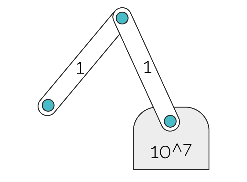
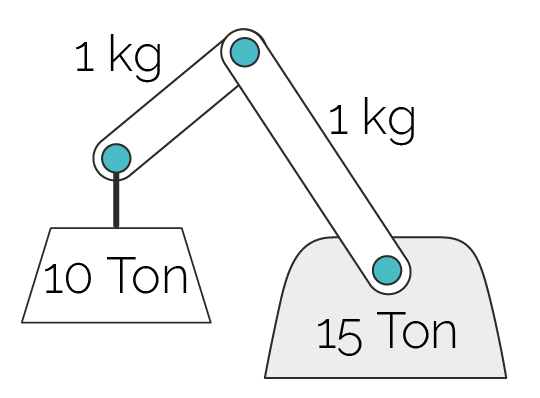
The direct method solves to machine precision. It can handle stiff systems with large conditions numbers and and huge mass ratios.
Physics based regularization of constraints eliminates the problem of over-constrained systems.
Linear elasticity is an integral part of the multibody model and enables realtime simulation of elastic components.
The model and solver are insensitive to mechanical singularities and simply reproduce the empirical behaviour.
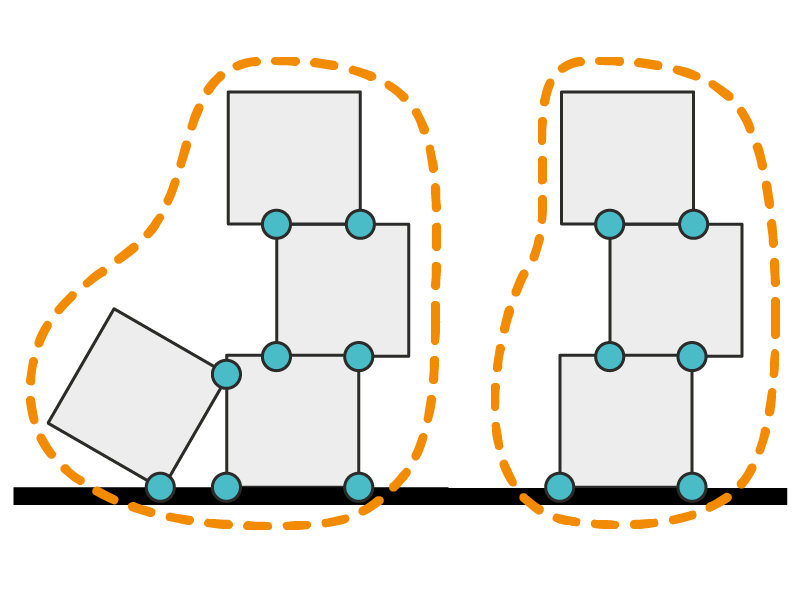
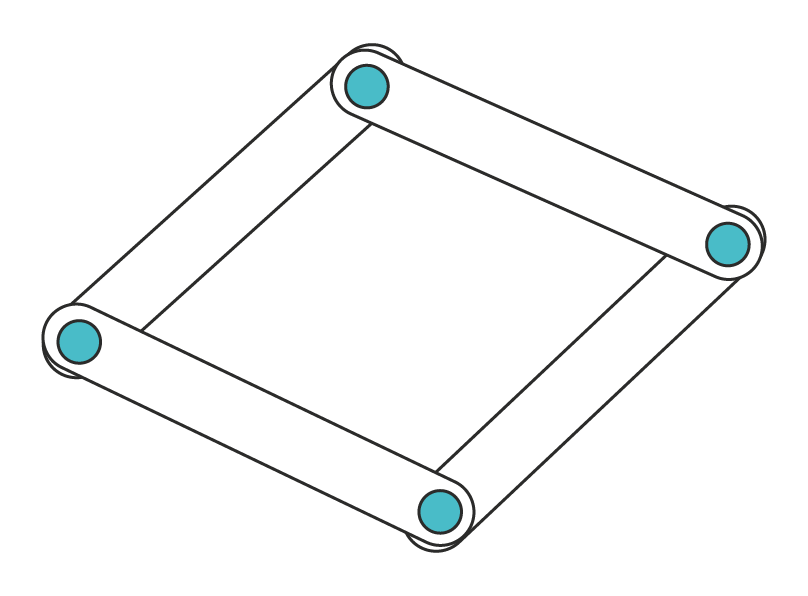
Grey – dynamic, blue – contacts, black – static
The solver automatically partitions the system for parallel solves of subsystems, which in turn also are parallelized.
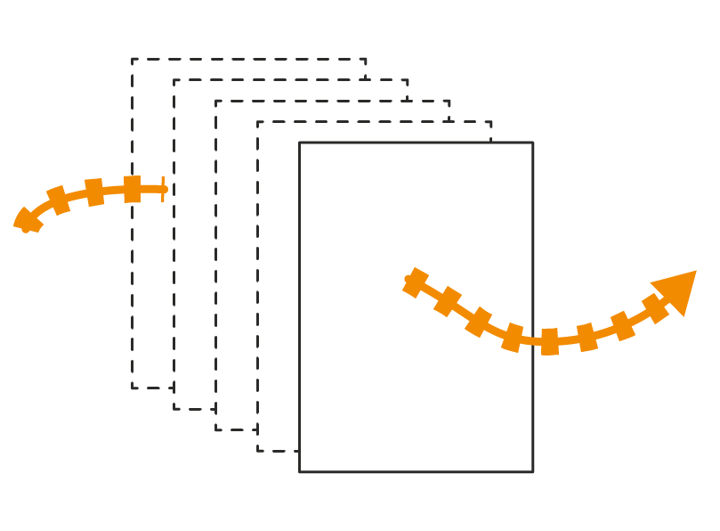
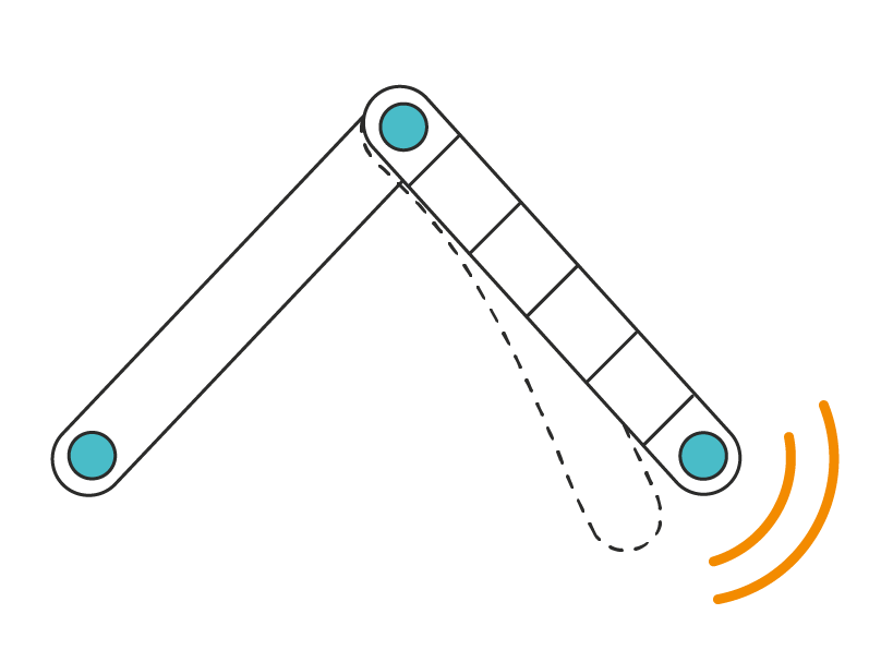
The symmetry preserving variational time integrator allows for large timesteps, even for very stiff systems.
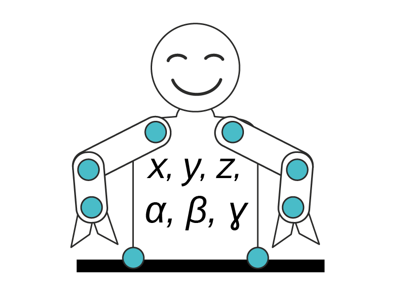
10 dynamic bodies = 60 DOF
Systems are solved with full- coordinate methods, which gives full dynamics and compliance and dissipation modeling in all degrees of freedom.